Small Area Estimation for Poverty Mapping
Contents
1. Small Area Estimation for Poverty Mapping#
The eradication of poverty, which was the first of the Millennium Development Goals (MDG) established by the United Nations and followed by the Sustainable Development Goals (SDG), requires knowing where the poor are located. Traditionally, household surveys are considered the best source of information on the living standards of a country’s population. Data from these surveys typically provide a sufficiently accurate direct estimate of household expenditures or income and thus estimates of poverty at the national level and larger international regions. However, when one starts to disaggregate data by local areas or population subgroups, the quality of these direct estimates diminishes. Consequently, National Statistical Offices (NSOs) cannot provide reliable wellbeing statistical figures at a local level. For example, the Module of Socioeconomic Conditions of the Mexican National Survey of Household Income and Expenditure (ENIGH in Spanish) is designed to produce estimates of poverty and inequality at the national level and for the 32 federate entities (31 states and Mexico City) with disaggregation by rural and urban zones, every two years, but there is a mandate to produce estimates by municipality every five years, and the ENIGH alone cannot provide estimates for all municipalities with adequate precision. This makes monitoring progress toward the Sustainable Development Goals more difficult.
Beyond the SDGs, poverty estimates at a local level are crucial for poverty reduction. Policymakers interested in poverty reduction and alleviation will often have a limited budget, and information on poverty at a local level can potentially improve targeting. The need for cost-effective disaggregated statistics makes it necessary to use indirect techniques for poverty estimation at a local level. To better understand the spatial distribution of poverty within countries, the World Bank has been producing poverty estimates at increasingly higher resolutions (poverty maps) since before the turn of the 21st century. A poverty map is the illustration of poverty rates on a map and is used to highlight the spatial distribution of poverty and inequality across a given country. Poverty mapping relies on Small Area Estimation (SAE) methods which are statistical tools that can be deployed to produce statistics for small areas with much better quality than those obtained directly from a sample survey.1
Small area techniques combine auxiliary information from censuses, registers, or other larger surveys to produce disaggregated statistics of sufficient precision where survey data alone is insufficient. The techniques achieve this by specifying some homogeneity relationships across areas; hence, they are based on the idea that “union is strength.” Despite small area estimation being useful for many indicators, the focus here is on small area methods used for poverty and related indicators derived from welfare.
Ending extreme poverty is one of the World Bank’s twin goals and poverty reduction is how the institution’s efforts are often gauged. Accurate estimates of poverty at a granular level are an essential tool for monitoring poverty reduction and spatial inequalities. The World Bank’s efforts to develop small area estimates of poverty can be traced back to the late 1990s. An initial effort by the institution was implemented by in an application in Ecuador and is the bedrock of what came after. Much of the research efforts on small area estimation within the World Bank came to a zenith in the early 2000s with the publication of the paper “Micro-level estimation of poverty and inequality” by Elbers et al. [2003]. The method came to be known as ELL, and for over a decade-and-a-half, it was the default method used for all poverty mapping conducted by the World Bank. The method’s popularity was spurred by the World Bank’s development of a software application called PovMap (Zhao [2006]).2 The software provided a user-friendly interface for practitioners and did not require knowledge of specialized programming languages. The PovMap software was followed nearly a decade after by a Stata version called sae (Nguyen et al. [2018]).3
The Guidelines to Small Area Estimation for Poverty Mapping (hereafter the Guidelines) come after more than two decades of poverty mapping by the World Bank. These guidelines on small area estimation are meant as a practical guide to enable practitioners working on small area estimation of poverty to make informed choices between the available methods and make them aware of the strengths and limitations of the methodologies at hand. The Guidelines are also presented for practitioners who wish to learn about updates to the software and methods used within the World Bank for small area estimation. The Guidelines are not meant to be an exhaustive presentation of the small area estimation literature, instead, they focus almost exclusively on poverty and are a practical guide for practitioners to assist them in navigating the multiple different small area techniques available.4 The methods include but are not limited to, those proposed by Elbers et al. [2003] that generated a lot of the early poverty mapping work at the World Bank, a number of subsequent refinements and improvements to the original ELL methodology, area-level models, and some ongoing research. The Guidelines advise readers on what may be the best approach for different poverty mapping projects and different sets of data constraints by reviewing the relevant literature and conducting simulation exercises that compare across available methodologies. It is expected that the Guidelines will become a valuable resource to practitioners working in the area of poverty mapping.
Before jumping into the Guidelines, a brief background to small area estimation is provided, as well as a decision tree aimed at practitioners (Fig. 1.1) who seek what may be the best approach given their context. After the brief background, the guidelines present direct estimates in Chapter 2: Direct Estimates. Area-level models are presented in Chapter 3: Area-level Models for Small Area Estimation, focusing on Fay-Herriot methods (Fay III and Herriot [1979]). Unit-level methods are presented in Chapter 4: Unit-level Models for Small Area Estimation, giving special attention to the approach from Elbers et al. [2003] as well as that of Molina and Rao [2010]. Chapter 5: Poverty Mapping in Off-Census Years, presents proposed alternatives for poverty mapping in off-census years beyond area-level models. Finally, Chapter 6: Model Diagnostics is devoted to model selection and other considerations. Throughout chapters 2–5 the pros and cons of the chapter’s corresponding approaches are noted.
1.1. A Brief Background to Small Area Estimation#
Small area estimates are often used to create a poverty map, but the two terms, Poverty Mapping and Small Area Estimation, should not be used interchangeably. Small area estimation is a set of methods used by National Statistical Offices (NSO) and other organizations to achieve estimates of acceptable quality for publication. As statistical information is disaggregated into smaller population subgroups, it will become noisier and will yield larger Coefficients of Variation (CV), which may exceed the threshold established by the NSO above which they will choose not to publish that specific estimate. Model-based small area estimation techniques incorporate auxiliary information from censuses, registers, geospatial data, or other large surveys, to produce estimates of much better quality, even for areas with very small sample sizes.
Model-based techniques are popular because they yield good quality estimates even for areas with very small sample sizes. Of course, to achieve this, one needs to make model assumptions, and these assumptions need to be validated using the available data (Molina et al. [2021]). Moreover, the quality of the model behind the estimates should be thoroughly evaluated and small area estimates should be accompanied by valid measures of their precision (Rao and Molina [2015]).
Among small area estimation methodologies, area-level models use only aggregate auxiliary information at the area level. Aggregated data are more readily available because it is typically not subject to confidentiality. These models have other advantages that come with aggregate data, such as lower sensitivity to unit-level outliers. The disadvantage of the area-level method is less detailed information than unit-level models, specifically at the microdata level. Perhaps the most popular area method is the one proposed by Fay III and Herriot [1979] which is discussed in more detail in Chapter 3: Area-level Models for Small Area Estimation of these Guidelines.
Unit-level models take advantage of detailed unit-record information, when such information is available. The models rely on detailed income/expenditure information from household surveys and a set of household-level characteristics in both a household survey and a population census to simulate household expenditures or incomes for each household in the population census data.5
The first unit-level model for small area estimation, discussed in more detail in Chapter 4: Unit-level Models for Small Area Estimation of these Guidelines, was proposed by Battese et al. [1988] to estimate county crop areas of corn and soybeans. That model, called hereafter the BHF Model, includes, apart from the usual individual errors, random effects for the areas representing the between-area heterogeneity or idiosyncrasy the available auxiliary variables cannot explain. These models might also include area-level (or contextual) variables and thus may incorporate much more information in the estimation process than area-level models. As noted by Robinson and others [1991], models with random effects belong to the general class of mixed models and are commonly used in other fields such as Biostatistics, Engineering, Econometrics, and additional Social Sciences.6
Model-based small area estimates rely on statistical models to establish a relationship between a dependent variable and a set of covariates. The covariates and the parameters obtained from the fitted model are then used to predict the dependent variable in the auxiliary data. In the context of small area estimates of poverty, under unit-level models, the dependent variable is typically consumption/expenditure or income and relies on properly replicating the welfare distribution. The simulated welfare distribution makes it possible to obtain well-being indicators, such as the FGT class of indicators (Foster et al. [1984]). In the case of area-level models, the dependent variable is the direct estimator of the same indicator for the area.
The ELL method falls under the class of methods based on unit-level models for small area estimation. The method relies on a BHF model specified at the household level and may also include area or sub-area-level (contextual) variables. At the time of publication, it was one of the first times a model relied on using microdata to simulate the welfare distribution, which allowed the calculation of numerous indicators beyond just area aggregates.7 The methodology quickly gained traction within the World Bank, as well as among National Statistical Offices around the world, and has been one of the most applied methods to obtain small area estimates. Since ELL’s publication, however, there have been considerable advances in the literature, including Molina and Rao’s (Molina and Rao [2010]) Empirical Best (EB) method.
When deciding which small area estimation method is preferable, there are many considerations the practitioner should take into account, but ultimately, the method chosen is often driven by the data at hand. When the practitioner has access to census data and a contemporaneous household survey, it is nearly always advisable to apply a unit-level model (Chapter 4: Unit-level Models for Small Area Estimation), because they often yield the most significant gains in precision. However, the data requirements for these models are considerable, and these data need to be checked to ensure the two data sources are also comparable beyond the temporal aspect. Potential variables need to be defined similarly in both data sources and must have similar distributions, as differences may lead to biased estimators. When choosing a unit-level model-based procedure, the next decision is often the aggregation level at which estimates will be reported. If there is a need for estimates at two different levels, then two-fold nested-error models may be used; otherwise one-fold nested-error models are adequate.
When unit-level models are not possible, area-level models may be a viable alternative (Chapter 3: Area-level Models for Small Area Estimation). Area-level models are often easier to implement than unit-level models since data requirements are minimal and may be used when census data and survey data are not contemporaneous or incongruous. Also, area-level models rely on aggregated data, which is often not subject to confidentiality. In addition, if the most recent census is too old for a unit-level model, the recommended approach is to consider an area-level model. The most popular area-level model for small area estimation is the Fay-Herriot (FH) model, introduced by Fay III and Herriot [1979], to estimate the per capita income of small areas in the United States. The U.S. Census Bureau has used area-level models within the Small Area Income and Poverty Estimates (SAIPE) project to inform the allocation of federal funds to school districts. The Fay-Herriot method, discussed in the area-level model chapter, will often require a separate model for each indicator, implying that area-level covariates are linearly related to the indicator of interest. If there is data at different aggregation levels, it may be possible to implement a two-fold area-level model introduced by Torabi and Rao [2014], although no software implementation is currently available. Alternatively, it is possible to perform an FH model at the lowest aggregation level, and aggregate these FH estimates to a higher level (see Section 3.4.1). Although area-level models predate ELL and in principle, should be simpler to execute, they have not been as commonly implemented by World Bank teams.
In addition to unit- and area-level models, unit-context models have been proposed in the context of SAE for poverty during off-census years (Chapter 5: Poverty Mapping in Off-Census Years). Unit-context models (Section 5.1) attempt to model the population’s welfare distribution by using only area-level covariates. This method may be attractive because it can rely on easily accessible aggregate data and may benefit from the larger sample size obtained via household-level welfare distribution and thus appears to combine the best features of both area-level and unit-level methodologies. Nevertheless, simulated data and real-world data have shown that unit-context models yield biased poverty estimates and, therefore, based on the literature to date, are discouraged and not considered preferable over estimators based on FH area-level models. Additionally, unit-context models rely on a parametric bootstrap procedure to estimate Mean Square Error (MSE). Given the assumptions of the unit-context model, that household-level welfare distribution does not depend on household-specific characteristics, it is unlikely that the MSE can be accurately estimated following a parametric bootstrap, making it difficult to evaluate the resulting small area estimates properly.
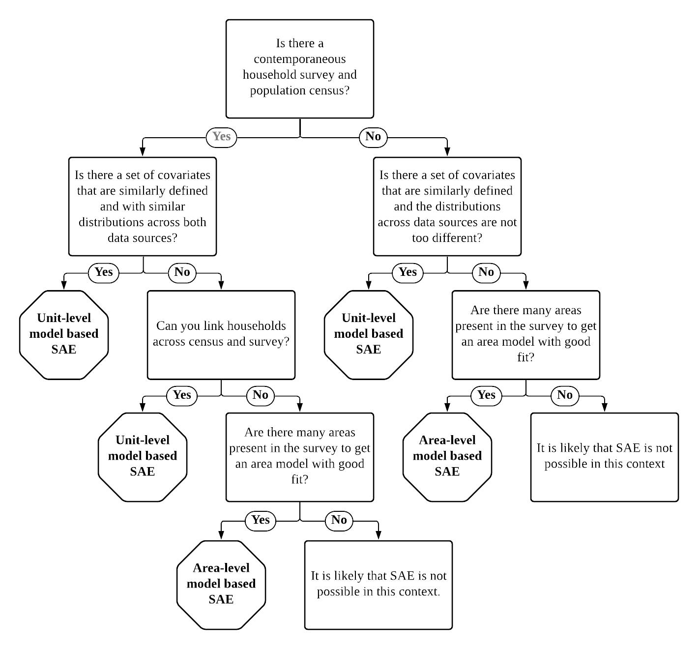
Fig. 1.1 SAE Decision tree#
Machine learning methods have also been proposed to obtain poverty maps in off-census years or when census data is unavailable. The methods often combine household survey data with ancillary Geo-coded (publicly available and proprietary) data to present local estimates of welfare. These methods have gained popularity among academia and policy circles since the publication of Jean et al. [2016]. For example, during the COVID-19 pandemic, cash transfers in Nigeria were informed by poverty estimates obtained from a machine learning approach by Chi et al. [2021]. However, these methods lack an accurate estimate of the method’s noise and, to date, have not been submitted to a rigorous statistical validation. The Guidelines present a brief look into how these machine learning methods compare to other available small area estimation approaches. Although much work remains to be done regarding machine learning methods, the Guidelines posit that these methods are promising (see Section 5.2).
As the reader delves into the Guidelines and cited literature, the complexity of which method to choose becomes apparent. Despite this caveat, a simple decision tree on method availability is presented in Fig. 1.1. This decision tree can be used to assist practitioners in choosing which model is the best route for their context. The decision tree simplifies the process by directing readers to specific chapters in the Guidelines relevant to their particular situation.
1.2. About the Guidelines#
The Guidelines are meant as a practical guide for readers. Stata scripts are provided throughout the chapters. These scripts allow replicating most sections and figures, which hopefully can assist new and more experienced practitioners in their SAE applications. Readers may download the latest Stata (SAE) packages used throughout the Guidelines from:
Unit-level models: https://github.com/pcorralrodas/SAE-Stata-Package
Area-level models: https://github.com/jpazvd/fhsae
Although R offers a wide variety of packages for poverty-related small area estimation these are described in other sources: Rao and Molina [2015], , Molina [2019], and , for example.
To assist readers throughout the text, simulated data (created following an assumed model), as well as real-world data are used. These data are used for method comparisons. Simulated data follow an assumed model and data generating process and are used for model-based simulations. Scripts are provided in the case of simulated data which can assist readers to replicate many of the analyses in the text. These data assist in illustrating the application of the different methods discussed and are used to make salient the advantages and disadvantages of the methods discussed.8 In addition to simulated data, the Guidelines use the Mexican Intercensal survey for design-based validations where methods are compared using real world-data and the real data generating process is unknown.9
1.3. References#
- BHF88
George E. Battese, Rachel M. Harter, and Wayne A. Fuller. An error-components model for prediction of county crop areas using survey and satellite data. Journal of the American Statistical Association, 83(401):28–36, 1988. URL: http://www.jstor.org/stable/2288915.
- CFCB21
Guanghua Chi, Han Fang, Sourav Chatterjee, and Joshua E Blumenstock. Micro-estimates of wealth for all low-and middle-income countries. arXiv preprint arXiv:2104.07761, 2021.
- CHMM21
Paul Corral, Kristen Himelein, Kevin McGee, and Isabel Molina. A map of the poor or a poor map? Mathematics, 2021. URL: https://www.mdpi.com/2227-7390/9/21/2780, doi:10.3390/math9212780.
- CMN21
Paul Corral, Isabel Molina, and Minh Cong Nguyen. Pull your small area estimates up by the bootstraps. Journal of Statistical Computation and Simulation, 91(16):3304–3357, 2021. URL: https://www.tandfonline.com/doi/abs/10.1080/00949655.2021.1926460, doi:10.1080/00949655.2021.1926460.
- Dem02
Gabriel Demombynes. A manual for the poverty and inequality mapper module. University of California, Berkeley and Development Research Group, the World Bank, 2002.
- ELL03(1,2,3)
Chris Elbers, Jean O Lanjouw, and Peter Lanjouw. Micro–level estimation of poverty and inequality. Econometrica, 71(1):355–364, 2003.
- FIH79(1,2,3)
Robert E Fay III and Roger A Herriot. Estimates of income for small places: an application of James-Stein procedures to census data. Journal of the American Statistical Association, 74(366a):269–277, 1979.
- FGT84
James Foster, Joel Greer, and Erik Thorbecke. A class of decomposable poverty measures. Econometrica: Journal of the Econometric Society, 52:761–766, 1984.
- JBX+16
Neal Jean, Marshall Burke, Michael Xie, W Matthew Davis, David B Lobell, and Stefano Ermon. Combining satellite imagery and machine learning to predict poverty. Science, 353(6301):790–794, 2016. URL: https://www.science.org/doi/abs/10.1126/science.aaf7894.
- Mol19(1,2)
Isabel Molina. Desagregación De Datos En Encuestas De Hogares: Metodologías De Estimación En áreas Pequeñas. CEPAL, 2019. URL: https://repositorio.cepal.org/handle/11362/44214.
- MCN21
Isabel Molina, Paul Corral, and Minh Cong Nguyen. Model-based methods for poverty mapping: a review. Unpublished manuscript, 2021.
- MR10(1,2)
Isabel Molina and JNK Rao. Small area estimation of poverty indicators. Canadian Journal of Statistics, 38(3):369–385, 2010.
- NCAZ18
Minh Cong Nguyen, Paul Corral, João Pedro Azevedo, and Qinghua Zhao. Sae: a stata package for unit level small area estimation. World Bank Policy Research Working Paper, 2018.
- RM15(1,2,3)
JNK Rao and Isabel Molina. Small Area Estimation. John Wiley & Sons, 2nd edition, 2015.
- R+91(1,2)
George K Robinson and others. That blup is a good thing: the estimation of random effects. Statistical science, 6(1):15–32, 1991.
- TR14
Mahmoud Torabi and JNK Rao. On small area estimation under a sub-area level model. Journal of Multivariate Analysis, 127:36–55, 2014.
- TZL+18
Nikos Tzavidis, Li-Chun Zhang, Angela Luna, Timo Schmid, and Natalia Rojas-Perilla. From start to finish: a framework for the production of small area official statistics. Journal of the Royal Statistical Society: Series A (Statistics in Society), 181(4):927–979, 2018.
- Zha06
Qinghua Zhao. User Manual for Povmap. 2006. URL: http://siteresources. worldbank. org/INTPGI/Resources/342674-1092157888460/Zhao_ ManualPovMap. pdf.
1.4. Notes#
- 1
There is no universal threshold used to define a small area; every NSO establishes its own limit of what is an acceptable coefficient of variation (CV). Anything above the threshold is unlikely to be published by the NSO. Moreover, there is also no defined sample size that can determine if a group can be considered a small area since this is also dependent on the indicator one wishes to estimate. For poverty, for example, the magnitude of the poverty rate is also related to the necessary sample size for its accurate estimation, with higher proportions requiring smaller sample sizes.
- 2
Demombynes [2002] presents earlier work of a module in SAS of the methodology.
- 3
Although
saewas initially created to replicate many of the features and methods implemented inPovMap, the package has undergone many updates. Corral et al. [2021] detail the main updates and the reasons behind these.- 4
For a more thorough discussion on small area estimation, including applications for other indicators of interest, readers should refer to Rao and Molina [2015].
- 5
Note that simulations are not required when using analytical formulas to obtain poverty estimates. When assuming normality, the expected value of the poverty headcount and gap can be calculated without resorting to Monte Carlo simulations (Molina [2019]).
- 6
Early applications were in the area of animal and plant breeding to estimate genetic merits (Robinson and others [1991]).
- 7
ELL follows and builds upon the work of .
- 8
See Tzavidis et al. [2018] for more details.
- 9
The Mexican Intercensal survey contains a welfare measure and is modified to mimic a census of 3.9 million households and 1,865 municipalities to allow for a design-based validation. From the created census, 500 survey samples were drawn for validations shown throughout the document (see Corral et al. [2021] for more details on the modifications to the Mexican Intercensal survey and the sampling approach taken).