Area-level Models for Small Area Estimation
Contents
3. Area-level Models for Small Area Estimation#
This chapter focuses on the application of the basic area-level models for small area estimation, using Fay and Herriot’s (Fay III and Herriot [1979]) model as an example. Following a brief introduction, the next section provides an example of an application of the Fay-Herriot Model for small area estimation. Then the advantages and disadvantages of the method are discussed. Finally, a technical appendix for the methodology is provided. This section draws heavily from Molina [2019] and Molina et al. [2021], and readers are advised to consult these texts for further information.
3.1. Overview#
In the context of poverty, methods based on area-level models typically rely on estimating the distribution of the target area-level poverty indicator, given a set of area-level covariates based on two models – a sampling model for direct area estimates of poverty and a linking model where the true indicator is linearly related to a vector of auxiliary variables across all areas (see Technical appendix in this chapter).
In contrast to unit-level methods, these methods do not require unit record (most commonly household level) census data since they use only auxiliary information aggregated to the area level. Not typically subject to confidentiality concerns, aggregated data are usually more available. Such is often the case with population census data, where aggregated estimates for localities may be readily available while the detailed household-level data are restricted. Beyond censuses, data from other sources, such as administrative records, remote sensing data, and previous census aggregates, may also be available at the level of the areas or can be readily aggregated to that level and may be included as covariates in an area-level model. Aggregated data are also less sensitive to unit-level outliers. However, if there is high heterogeneity within the geographic units at which the area models are estimated, these benefits are balanced by a substantial loss of information when unit record level data are aggregated. Ultimately, whether unit record-level models offer a greater degree of precision depends on the explanatory power of the covariates that can be included in the area-level and unit-level models.
The most popular area-level model is the Fay-Herriot (FH) model, introduced by Fay III and Herriot [1979] to estimate the mean per capita income in small places in the United States of America (USA). The U.S. Census Bureau has regularly used it within the Small Area Income and Poverty Estimates (SAIPE) project to produce estimates for counties and states of the total number of people in poverty by age groups, household median income, and mean per capita income (see Bell [1997]). The U.S. Department of Education uses these estimates to determine annual allocations of federal funds given to school districts. Several other studies have employed area-level models to obtain poverty estimates in small areas around the world. Molina and Morales [2009] used these models to obtain estimates for Spanish provinces, Corral and Cojocaru [2019] in Moldova, Casas-Cordero Valencia et al. [2016] in Chile, as well as Seitz [2019] which applies the FH model to obtain district-level estimates of poverty in Central Asian countries.
Extensions of the basic FH model to account for temporal and spatial correlation have also been considered in the poverty mapping context, although not explored in these Guidelines. Interested readers may refer to Esteban et al. [2012] and Esteban et al. [2012], who used the FH model with temporal correlation first proposed by to estimate small area poverty indicators. used a spatial FH model to estimate mean income and poverty rates for the 57 Labor Local Systems of the Tuscany region in Italy for the year 2011. considered a spatio-temporal model to estimate poverty indicators for Spanish provinces in 2008, making use of survey data from the years 2004-2008.
3.2. Conducting Your First SAE Application with the Fay-Herriot Model#
The first step towards obtaining small area estimates based on the FH model is to compute direct estimates. For the purpose of this exercise, a 1 percent SRS sample within municipalities was drawn from the Mexican intracensal survey of 2015 (Encuesta Intercensal). To obtain direct estimates with correctly calculated standard errors from a complex sample, it is necessary to input the structure by specifying the stratification and clustering used. Complex survey designs usually include a minimum of two clusters per stratum to permit the estimation of sampling variance using standard procedures, but as SAE reports results for areas below which the sample was originally designed, there may be areas represented in the sample by just one PSU; in such cases, the usual variance estimates cannot be computed and it may be necessary to obtain an estimate of the sampling variance via alternative methods. This is a clear limitation of the FH method.1 Another limitation of the method is that, in locations with small sample size, everyone may be poor or no one is poor, which leads to an estimated variance of 0. In this case, the FH model is not directly applicable in those locations unless another method is used to predict those variances. The Stata script below describes how to obtain direct estimates of poverty rates \(\hat{\tau}_{d}^{DIR}\) and their sampling variances \(\psi_{d}\) for each location \(d\) in the sample:
clear all
set more off

/*==============================================================================
Do-file prepared for SAE Guidelines
- Real world data application
- authors Paul Corral
*==============================================================================*/

global main     "C:\Users\\`c(username)'\OneDrive\SAE Guidelines 2021\"
global section  "$main\2_area_level\"
global mdata    "$section\1_data\"
global survey   "$mdata\Survey_1p_mun.dta"
global povline = 715

version     15
set matsize 8000
set seed    648743

*===============================================================================
// End of preamble
*===============================================================================
//load in survey data
use "$survey", clear
	//Population weights and survey setup
	gen popw = Whh*hhsize

	//FGT
	forval a=0/2{
	    gen fgt`a' = (e_y<${povline})*(1-e_y/(${povline}))^`a'
	}

	//SVY set, SRS
	svyset [pw=popw], strata(HID_mun)
	//Get direct estimates
	qui:svy: proportion fgt0, over(HID_mun)
	//Extract poverty rates and  (1,865 Municipalities) - ordered from
	//smallest HID_mun to largest HID_mun
	mata: fgt0     = st_matrix("e(b)")
	mata: fgt0     = fgt0[1866..2*1865]'
	mata: fgt0_var = st_matrix("e(V)")
	mata: fgt0_var = diagonal(fgt0_var)[1866..2*1865]
	//Our survey already has the area level means of interest obtained from
	// the census. Leave data at the municipality level.
	gen num_obs = 1
	groupfunction [aw=popw], rawsum(num_obs) mean(poor fgt0) first(mun_*) by(HID_mun)
	sort HID_mun //ordered to match proportion output

	//Pull proportion's results
	getmata dir_fgt0 = fgt0 dir_fgt0_var = fgt0_var
	replace dir_fgt0_var = . if dir_fgt0_var==0
	replace dir_fgt0     = . if missing(dir_fgt0_var)


save "$mdata\direct.dta", replace
With the direct survey estimates \(\hat{\tau}_{d}^{DIR}\) of the indicators \(\tau_{d}\) in hand, it is possible to produce new estimates of \(\tau_{d}\) based on the fitted model. This model takes as an input, apart from the direct estimates for each location, \(\hat{\tau}_{d}^{DIR}\), their corresponding (heteroskedastic) sampling variances \(\psi_{d}\), which are assumed known, and the aggregated values of the covariates \(\mathbf{x}_{d}\). This information is used to estimate the FH regression coefficients \(\beta\) and the variance of the area effects \(u_{d}\), \(\sigma_{u}^{2}\). There are multiple approaches to predict the unknown random effects of the model, \(u_{d}\), in Equation (3.1). Stata’s fhsae package (Corral et al. [2018])2 obtains estimates similar to those provided from the eblupFH() function of Molina and Marhuenda [2015] R sae package, while the fayherriot package in Stata by Halbmeier et al. [2019] is an excellent alternative since it offers transformations to the data to ensure the assumptions of the model are met. The available model-fitting methods in the fhsae package are maximum likelihood (ML), restricted maximum likelihood (REML), and an approach presented by Fay III and Herriot [1979] based on the method of moments. As noted by Molina [2019], REML corrects the ML estimate of \(\sigma_{u}^{2}\) by the degrees of freedom due to estimating the regression coefficients, \(\beta\), and yields a less biased estimator in finite samples; thus REML is used in the example below.
The final estimate of the target indicator \(\tau_{d}\) is the empirical best linear unbiased (EBLUP) predictor of \(\tau_{d}\) under the FH model. This estimator uses the estimated value \(\hat{\sigma}_{u}^{2}\) of \(\sigma_{u}^{2}\) and can be expressed as a weighted average between the direct estimator and the regression-synthetic estimator \(\mathbf{x}'_{d}\hat{\beta}\) as noted by Rao and Molina [2015]. The final EBLUP referred to as FH estimator, is given by \(\hat{\tau}_{d}^{FH}=\hat{\gamma}_{d}\hat{\tau}_{d}^{DIR}+\left(1-\hat{\gamma}_{d}\mathbf{x}'_{d}\hat{\beta}\right)\). In this estimator, the weight attached to the direct estimator \(\hat{\tau}_{d}^{DIR}\) is given by \(\hat{\gamma}_{d}=\frac{\hat{\sigma}_{u}^{2}}{\hat{\sigma}_{u}^{2}+\psi_{d}}\) which lies between 0 and 1 and decreases in the error variance, \(\psi_{d}\). In locations \(d\) with small sample size and consequently where the direct estimator has a large sampling variance, \(\psi_{d},\) or when the auxiliary information in the model yields good explanatory power, a higher weight is assigned to the corresponding synthetic estimator.
The script illustrating model selection and small area estimation based on FH is provided below. Although there are options such as stepwise or lasso regression, it is preferable to use methods that consider the random effects (Lahiri and Suntornchost [2015]). The method for variable selection used in the script considers the random effects and is similar in spirit to a stepwise regression. Initially, the random effect model is fit including all the covariates. Due to lower computational requirements, the process employs the feasible generalized least squares (FGLS) method from Chandra et al. [2013]. Non-significant covariates are removed from the model sequentially, starting with those with the largest p-values.3 Then, from the remaining covariates, those with a variance inflation factor (VIF) above five are similarly removed. Finally, it is also essential to check that the model’s assumptions hold. In this case, the model residuals are relatively well aligned to the theoretical quantiles of a normal distribution, although some outliers are present (Fig. 3.1).
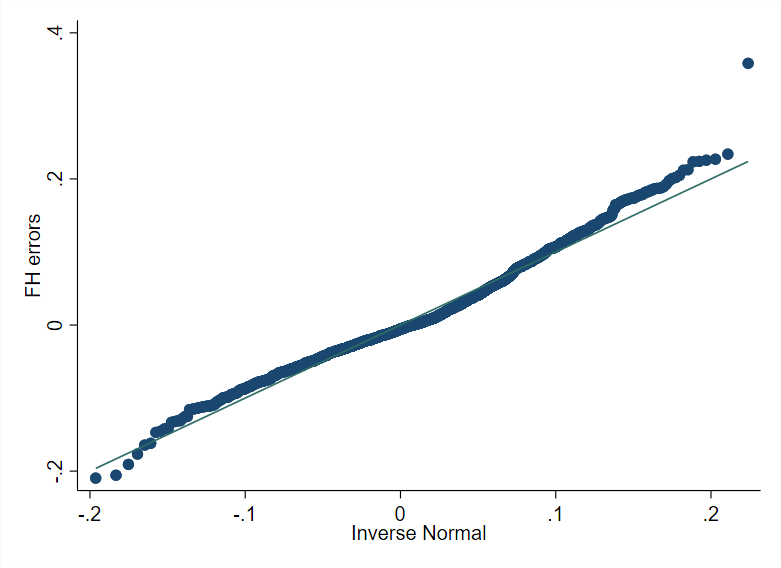
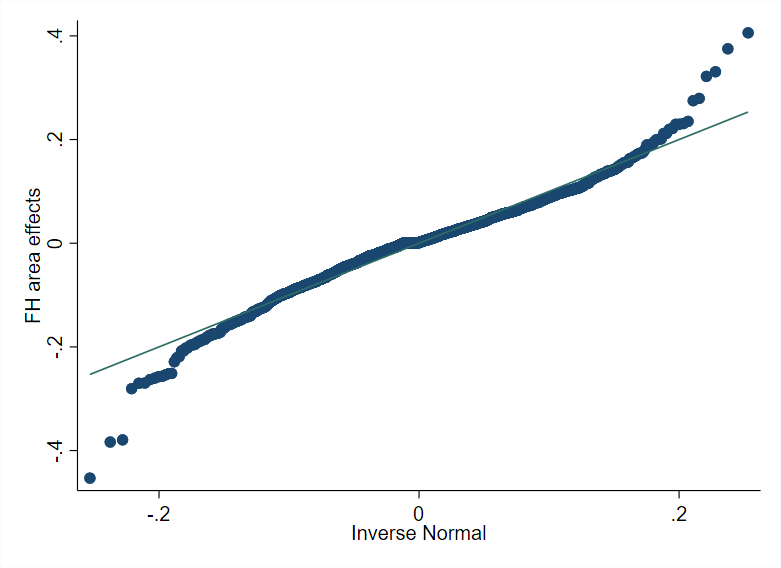
Fig. 3.1 Fay-Herriot model residuals (left) and predicted area effects (right)#
Source: Based on a 1% SRS sample by municipality of Mexican Intercensal survey of 2015. The figure on the left presents a normal q-q plot where the empirical quantiles of the standardized residuals from the FH model are plotted against the theoretical quantiles of the normal distribution. The figure on the right plots the empirical quantiles of the predicted area effects against the theoretical quantiles of the normal distribution.
clear all
set more off

/*==============================================================================
Do-file prepared for SAE Guidelines
- Real world data application
- authors Paul Corral
*==============================================================================*/

global main     "C:\Users\\`c(username)'\OneDrive\SAE Guidelines 2021\"
global section  "$main\2_area_level\"
global mdata    "$section\1_data\"
global survey "$mdata\Survey_1p_mun.dta"
global povline = 715
//Global with eligible variables
global thevar mun_hhsize mun_age_hh mun_male_hh mun_piped_water ///
mun_no_piped_water mun_no_sewage mun_sewage_pub mun_sewage_priv ///
mun_electricity mun_telephone mun_cellphone mun_internet ///
mun_computer mun_washmachine mun_fridge mun_television mun_share_under15 ///
mun_share_elderly mun_share_adult mun_max_tertiary mun_max_secondary ///
mun_share_female

version     15
set matsize 8000
set seed    648743

*===============================================================================
// End of preamble
*===============================================================================
use "$mdata\direct.dta", clear

	//Fit full model
	fhsae dir_fgt0 $thevar, revar(dir_fgt0_var) method(fh)

	local hhvars $thevar

	//Removal of non-significant variables
	forval z= 0.8(-0.05)0.0001{
		qui:fhsae dir_fgt0 `hhvars', revar(dir_fgt0_var) method(fh)
		mata: bb=st_matrix("e(b)")
		mata: se=sqrt(diagonal(st_matrix("e(V)")))
		mata: zvals = bb':/se
		mata: st_matrix("min",min(abs(zvals)))
		local zv = (-min[1,1])
		if (2*normal(`zv')<`z') exit
		foreach x of varlist `hhvars'{
			local hhvars1
			qui: fhsae dir_fgt0 `hhvars', revar(dir_fgt0_var) method(fh)
			qui: test `x'
			if (r(p)>`z'){
				local hhvars1
				foreach yy of local hhvars{
					if ("`yy'"=="`x'") dis ""
					else local hhvars1 `hhvars1' `yy'
				}
			}
			else local hhvars1 `hhvars'
			local hhvars `hhvars1'
		}
	}

	//Global with non-significant variables removed
	global postsign `hhvars'
	//Final model without non-significant variables
	fhsae dir_fgt0 $postsign, revar(dir_fgt0_var) method(fh)
	//Check VIF
	reg dir_fgt0 $postsign, r
	gen touse = e(sample)
	gen weight = 1
	mata: ds = _f_stepvif("$postsign","weight",5,"touse")
	global postvif `vifvar'

	local hhvars $postvif

	//One final removal of non-significant covariates
	forval z= 0.8(-0.05)0.0001{
		qui:fhsae dir_fgt0 `hhvars', revar(dir_fgt0_var) method(fh)
		mata: bb=st_matrix("e(b)")
		mata: se=sqrt(diagonal(st_matrix("e(V)")))
		mata: zvals = bb':/se
		mata: st_matrix("min",min(abs(zvals)))
		local zv = (-min[1,1])
		if (2*normal(`zv')<`z') exit
		foreach x of varlist `hhvars'{
			local hhvars1
			qui: fhsae dir_fgt0 `hhvars', revar(dir_fgt0_var) method(fh)
			qui: test `x'
			if (r(p)>`z'){
				local hhvars1
				foreach yy of local hhvars{
					if ("`yy'"=="`x'") dis ""
					else local hhvars1 `hhvars1' `yy'
				}
			}
			else local hhvars1 `hhvars'
			local hhvars `hhvars1'
		}
	}

	global last `hhvars'

	//Obtain SAE-FH-estimates
	fhsae dir_fgt0 $last, revar(dir_fgt0_var) method(reml) fh(fh_fgt0) ///
	fhse(fh_fgt0_se) fhcv(fh_fgt0_cv) gamma(fh_fgt0_gamma) out

	//Check normal errors
	predict xb
	gen u_d = fh_fgt0 - xb
		lab var u_d "FH area effects"

	histogram u_d

	gen e_d = dir_fgt0 - fh_fgt0
		lab var e_d "FH errors"

	histogram e_d


save "$mdata\direct_and_fh.dta", replace
If no transformation is applied in the model the FH estimates of the poverty rates may be negative for some areas. For those areas, the recommendation is to not use those negative FH estimates.4
As can be seen from Fig. 3.2, FH estimates are aligned to direct estimates. This figure also illustrates the larger adjustment made to direct estimates in locations where the sampling variance is larger. The resulting FH estimates also have a lower estimated root mean squared error (RMSE) than that of the direct estimates, suggesting an improved efficiency of the model-based estimates (Fig. 3.2, right).
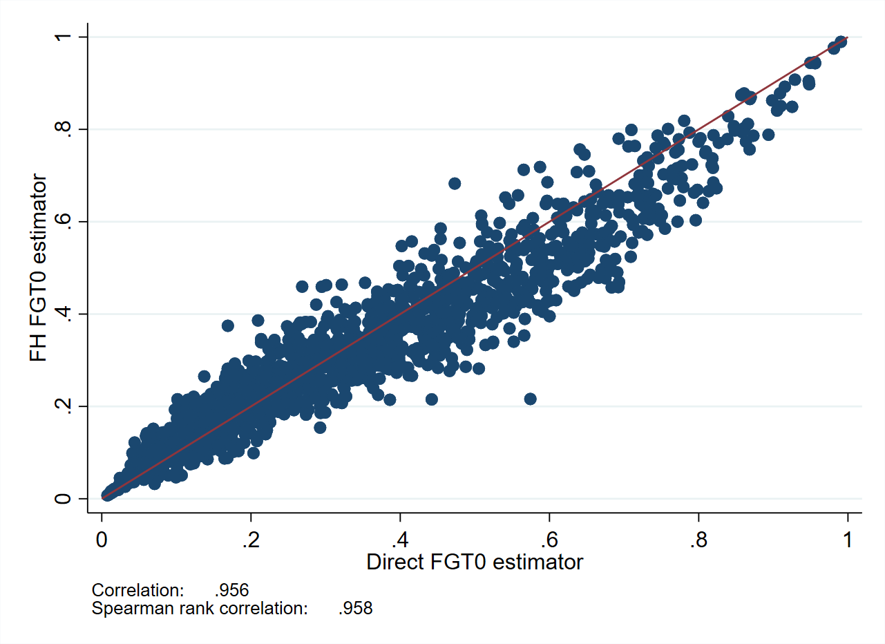
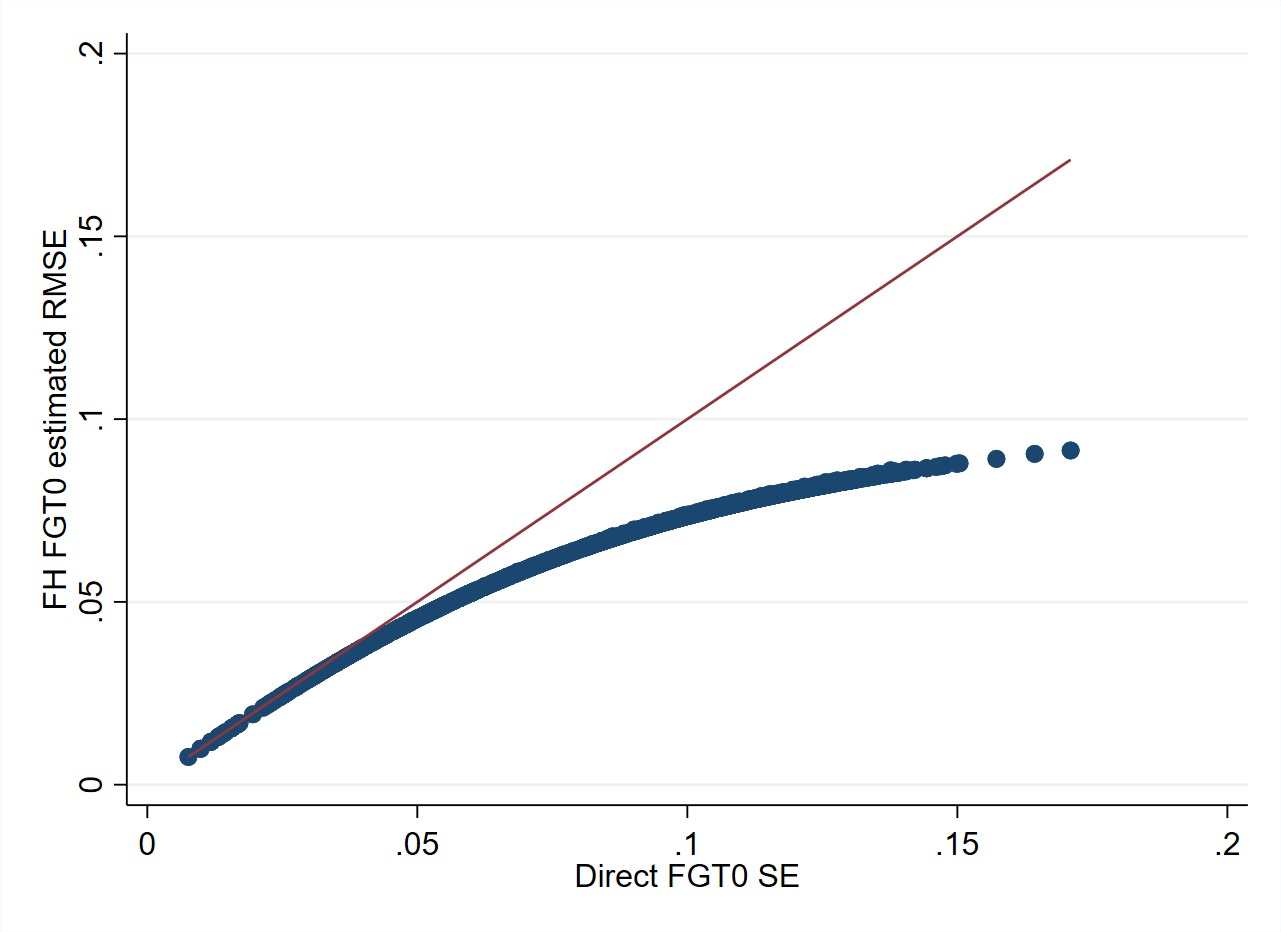
Fig. 3.2 FH poverty estimates compared to direct estimates#
Source: Based on a 1% SRS sample by municipality of Mexican Intercensal survey of 2015. The figure on the left presents a scatter plot of direct estimates on the X-axis and FH estimates on the Y-axis. The FH approach will often yield estimates that are highly aligned to the direct estimates.
The figure on the right illustrates the gains in terms of root mean squared error for the FH estimates (Y-axis) versus the standard error of the direct estimates (X-axis). Gains are often larger for the areas with smaller sample sizes (larger sampling errors of direct estimates), and though most if not all areas typically see some gains in precision.
3.3. Pros and Cons of Fay-Herriot Models#
The information in this section borrows heavily from Molina [2019] while adding more information on relevant aspects.
Model requirements:
Direct estimates of indicators of interest and its sampling variance for the areas considered, \(\hat{\tau}_{d}^{DIR}\) and \(\hat{\psi}_{d}\) respectively (from the survey).
Aggregate data at area level of all necessary covariates for the model for every area considered, \(\mathbf{x}_{d}\), \(d=1,\ldots,D\).
Pros:
Tend to improve the direct estimates in terms of efficiency (MSE).
The regression model incorporates unexplained heterogeneity between areas through the area effects.
The FH estimator is a weighted average of the direct estimator and the regression synthetic estimator (i.e., obtained by a linear regression). For areas where the sample size is small or where direct estimators have considerable sampling variance, the synthetic estimator will be given a higher weight. Accordingly, the FH estimate will approximate the direct estimate in areas with a sufficient sample .
Since the FH estimates make use of the direct estimates, which consider sampling weights with \(\gamma_{d}\) tending to one as the area sample size increases, it is consistent under the sampling design. Hence, provided that the sampling weights are accurate, FH estimates will be less affected by informative sampling (i.e., when the selection of the units for the sample depends on the outcome values - Rao and Molina [2015].
Since area-level aggregates are used, the final estimates are less affected by outliers.
Can provide estimates for non-sampled areas based on the regression-synthetic component.
The Prasad-Rao MSE estimates () are approximately unbiased. This holds as long as a sufficient number of areas are present and model assumptions are met, with normality for random effects and model errors.
It is easy and computationally fast to implement; considerably faster than unit-level models because the number of areas is typically much smaller than the actual sample size in typical unit-level models, and Monte Carlo or bootstrap methods are not necessary.
Does not require comparison of auxiliary variables between the different data sources to consider their use in the model.
Because aggregate data are used, confidentiality restrictions do not hinder the data acquisition process.
Cons:
Estimates are based on a model; thus, the model needs to be checked. For non-linear parameters (like poverty), the linear assumption of the model can be problematic.
The sampling variances of the direct estimates are assumed to be known, and the error of estimating these is not usually incorporated in the final estimates’ estimated MSE.
The Prasad-Rao MSE estimator () is approximately unbiased under the model with normality but is not design unbiased for a given area.
The model is fit only on sampled areas, which can be a very small number out of the total number of areas using only one observation by area (the direct estimator). As a consequence, model parameter estimators will be much less efficient than those obtained under unit-level models, and hence gains in precision are expected to be lower than those of estimators based on unit-level models.
Every indicator requires its own model.
Once estimates are obtained, these cannot be further disaggregated unless a new model at that level is constructed.
May require benchmarking adjustment to match direct estimates at higher aggregation levels. Although sub-area-level models by Torabi and Rao [2014] could be used to obtain estimates that naturally match at two different aggregation levels (different from the national level), user-friendly software is still not available.
3.3.1. Alternative Software Packages for Area-Level Models and Extensions#
In this section, the focus has been on Stata’s fhsae package. However, there is a wide variety of packages available in R for small area estimation based on the basic FH area-level model and on some extensions of this model proposed in the literature. Below is a list of some of these extensions of the FH model and the corresponding software implementation:5
The extension of the FH model proposed by that incorporates temporal correlation is implemented in the
saerypackage in R by . R’ssaepackage by Molina and Marhuenda [2015] includes a FH model with temporal and spatial correlation. Spatial correlation is also included in R’semdipackage ().Robust alternatives to the basic FH model, as well as its extensions, including spatial and temporal correlation, are detailed in and implemented in R’s
saeRobustpackage (). The robust spatial correlation model is also available in theemdipackage in R ().
In applications with several dependent target indicators, multivariate versions of the FH model may help provide even more efficient estimators. A multivariate version of the FH model was originally proposed by Fay [1987], and has been used to improve the estimates of median income of four-person families by using direct estimators of median income for three and five-person families by Datta et al. [1991] and Datta et al. [1996]. Multivariate FH models can be fitted with the R package
msae().The basic FH model assumes that covariates are population aggregates measured without error. For cases where auxiliary variables are measured with error, offer an extension to the basic FH model to account for the measurement error. Measurement error models can be applied with the R package
saeME(). This extension is also available in the R packageemdi().Hierarchical Bayesian methods have been applied
hbsaeR package by Boonstra [2015]. TheBayesSAER package (Shi ) also includes Bayesian extensions.Halbmeier et al. [2019] introduced the
fayherriotStata command, which allows for adjusting non-positive random effect variance estimates, and allows for transformation of the variable of interest to deal with violations of the model’s assumptions. Transformation is also available in theemdipackage in R ().
3.4. Technical Annex#
The FH model is defined in two stages.6 In the first stage, the true values of the indicators \(\tau_{d}\) for all the areas \(d=1,\ldots,D\), are linked by establishing a common linear regression model, called the linking model, where the true indicator is linearly related to a vector of area-level covariates \(\mathbf{x}_{d}\),
The random errors in this regression model, \(u_{d}\), are called area effects, because they represent the unexplained between-area heterogeneity. They are assumed to satisfy usual regression assumptions, such as having zero mean and constant variance \(\sigma_{u}^{2}\), which is typically unknown. Note that the linear regression model Equation (3.1) cannot be fitted to the data, because true values of the indicators \(\tau_{d}\) are not observed. Direct estimators \(\hat{\tau}_{d}^{DIR}\) of the indicators are available from the survey microdata but are, obviously, subject to survey error, since they are calculated only with the area-specific survey data, which is of small size. Hence, in the second stage, this survey error is modeled by assuming that the direct estimators are centered around the true values of the indicators, as follows:
with heteroscedastic errors, where error variances are \(\mathrm{var\left(\mathit{e_{d}|\tau_{d}}\right)=\psi_{\mathit{d}}}\), \(d=1,\ldots,D\), which is called the sampling model. Note that the \(D\) error variances \(\psi_{d}\), \(d=1,\ldots,D\), need to be assumed as known even if they are not; otherwise, there would be more unknown parameters than the available observations: \(\hat{\tau}_{d}^{DIR}\), \(d=1,\ldots,D\). These error variances are customarily estimated based on the survey microdata from the area of interest and perhaps smoothed afterward since these estimates are highly unstable due to the small area sample sizes.
The usual small area estimator obtained from this model is based on the best linear unbiased predictor (BLUP), which is defined as the linear function \(\hat{\tau}_{d}=\mathbf{\mathbf{\alpha}'y}\) of the data \(\mathbf{y}=(\hat{\tau}_{1}^{DIR},\ldots,\hat{\tau}_{D}^{DIR})'\), where \(\mathbf{\boldsymbol{\alpha}}=(\alpha_{1},\ldots,\alpha_{D})'\), which is unbiased under the model, that is, \(E(\hat{\tau}_{d}-\tau_{d})=0\), and is optimal (or best) in the sense of minimizing the mean squared error (MSE). The resulting BLUP \(\hat{\tau}_{d}\) of \(\tau_{d}\) can be expressed as a weighted average of the direct estimator \(\hat{\tau}_{d}^{DIR}\) and the regression-synthetic estimator, \(\mathbf{x}'_{d}\hat{\beta}\), where the weight \(\gamma_{d}=\sigma_{u}^{2}/(\sigma_{u}^{2}+\psi_{d})\) attached to the direct estimator grows as the error variances \(\psi_{d}\) decrease (or the area sample size increases), or the unexplained variation \(\sigma_{u}^{2}\) grows. This means that, in areas with a large sample size or when the auxiliary information is not very powerful, the FH estimates come close to the direct estimators; in the opposite case, they come close to the regression-synthetic estimators. This leads to the BLUP automatically borrowing strength only when it is actually needed and approximating to the conventional survey direct estimators when the area sample size is large or the model is not useful.
The BLUP does not require normality assumptions on the model errors or area effects, and it is unbiased under the model. The empirical BLUP (EBLUP) is obtained by replacing the unknown area effects’ variance \(\sigma_{u}^{2}\) by an estimator \(\hat{\sigma}_{u}^{2}\) with good properties (i.e. consistent). The EBLUP preserves unbiasedness under symmetric distributions and under certain regularity assumptions on the considered estimator \(\hat{\sigma}_{u}^{2}\) of \(\sigma_{u}^{2}\) (and a translation invariant function of the sample data \(\mathbf{y}\)), which are satisfied by the usual estimators obtained by ML, REML, or Fay-Herriot’s method of moments. However, their exact mean squared error (MSE) does not have a closed form. For this reason, analytical approximations with good properties for large number of areas \(D\) have been obtained under normality. Similarly, an analytical estimator of the true MSE that is nearly unbiased for large \(D\) has been obtained under normality. This MSE estimator depends on the actual estimator of \(\sigma_{u}^{2}\) that is applied; for the exact formulas, see Rao and Molina [2015], Section 6.2.1. For areas with moderate or large sample sizes and indicators (and corresponding direct estimators) defined in terms of sums over the area units, the normality assumption is minimally ensured by the Central Limit Theorem. However, for areas with small sample sizes or when target indicators are not defined in terms of sums over the area units, the normality assumption should be validated if these customary MSE estimates are considered; otherwise, they should be interpreted with care.
A problem that may occur when applying FH models is that the estimated model variance \(\sigma_{u}^{2}\) may be non-positive, and then it is customary to set it to zero. In these instances, the weight \(\gamma_{d}\) is equal to 0 for all areas, implying a weight of zero to direct estimates regardless of the area’s sample size. Hence, the EBLUP reduces to the synthetic estimator, which may be considerably different to the direct estimator (Rao and Molina [2015]). and propose adjustments to the maximum likelihood approach to obtain strictly positive estimates. These adjustments are incorporated into the emdi package in R ().
A clear drawback of the FH model is that the sampling variances of direct estimators, \(\psi_{d}\), \(d=1,\ldots,D\), are assumed to be known even if they are actually estimated,7 and usual MSE estimators do not account for the uncertainty due to estimation of these variances. Note also that, if one wishes to estimate several indicators, a different model needs to be constructed for each indicator, even if they are all based on the same welfare variable. This means that one needs to find area-level covariates that are linearly related to each indicator. It seems more reasonable to fit a model for the considered welfare variable at the unit-level and then estimate all the target monetary indicators based on that same model, as is done in the procedures based on unit-level models described in Chapter 4: Unit-level Models for Small Area Estimation.
Moreover, the area-level auxiliary information commonly has the shape of area means or proportions. For indicators with a more complex shape than the simple mean welfare, it might be difficult to find area-level covariates that are linearly related with the complex function of welfare for the area; consequently, the linearity assumption in the FH model might fail, and finding an adequate transformation for linearity to hold might not be easy in some applications. In any case, even if the gains obtained using the FH model depend on the explanatory power of the available covariates, Molina and Morales [2009] observed very mild gains of the EBLUPs of poverty rates and gaps based on the FH model in comparison to those obtained by Molina and Rao [2010] using the same data sources, but relying on unit-level models (and using the microdata). When considering indicators, such as the FGT poverty indicators, an additional drawback of the FH model is that due to the small area sample sizes, direct estimators that are equal to zero or one are possible (when no one or everyone is found to be below the poverty line), even if the area sample size is not zero. In those areas, the sampling variances of the direct estimators are also zero and unless a different approach is applied to obtain strictly positive variances, the FH Model is not applicable for those areas. A common approach to correct for this is to remove those areas in the modeling phase and then use a synthetic estimator for that area instead.
3.4.1. Aggregation to Higher Geographic Areas#
Even if the area-level model may be applied to produce poverty estimates at a given level of aggregation, one may also wish to aggregate these estimates to higher aggregation levels (let us call these larger areas “regions”). While the estimate of the poverty rate for a region is simply the population weighted average of the area-level poverty rates contained within the region, obtaining a correct MSE estimate for the estimator of that region requires aggregating the estimates of the MSEs and mean crossed product errors (MCPEs) at the area level, \(d\), up to the regional level, \(r\). For a region, \(r\), containing \(D_{r}\) areas, the poverty rate is then \(\tau_{r}=\frac{1}{N_{r}}\sum_{d=1}^{D_{r}}N_{d}\tau_{d}\), where \(\tau_{d}\) is the poverty rate in area \(d\), from region \(r\), \(N_{d}\) is the population of domain \(d\) in region \(r\), and \(N_{r}=\sum_{d=1}^{D_{r}}N_{d}\) the population of the region. Then a model-based estimate of the poverty rate for region \(r\) is \(\hat{\tau}_{r}=\frac{1}{N_{r}}\sum_{d=1}^{D_{r}}N_{d}\hat{\tau}_{d}\), and the MSE of \(\hat{\tau}_{r}\) is given by:
where \(MCPE\left(\hat{\tau}_{d},\:\hat{\tau}_{l}\right)=E\left[\left(\hat{\tau}_{d}-\tau_{d}\right)\left(\hat{\tau}_{l}-\tau_{l}\right)\right]\) (Rao and Molina [2015], p144). The fhsae package in Stata has the option to apply such an approach via its aggarea() option. The method is also available in the hbsae R package by Boonstra [2015].
3.5. References#
- Bel97
W Bell. Models for county and state poverty estimates. Preprint, Statistical Research Division, US Census Bureau, 1997.
- Boo15(1,2)
Harm Jan Boonstra. Package 'hbsae'. R Package Version, 2015.
- CCVEL16
Carolina Casas-Cordero Valencia, Jenny Encina, and Partha Lahiri. Poverty mapping for the Chilean Comunas. Analysis of Poverty Data by Small Area Estimation, pages 379–404, 2016.
- CSG13
Hukum Chandra, UC Sud, and VK Gupta. Small area estimation under area level model using r software. New Delhi: Indian Agricultural Statistics Research Institute, 2013.
- CC19
Paul Corral and Alexandru Cojocaru. Moldova poverty map: an application of small area estimation. mimeo. Unpublished manuscript, 2019.
- CSAN18
Paul Corral, William Seitz, João Pedro Azevedo, and Minh Cong Nguyen. FHSAE: Stata module to fit an area level Fay-Herriot model. Statistical Software Components. 2018. URL: https://econpapers.repec.org/software/bocbocode/s458495.htm.
- DFG91
Gauri S Datta, RE Fay, and M Ghosh. Hierarchical and empirical multivariate bayes analysis in small area estimation. In Proceedings of bureau of the census 1991 annual research conference, US Department of Commerce, Bureau of the Census, volume 7, 63–79. 1991.
- DGNN96
GS Datta, Malay Ghosh, Narinder Nangia, and K Natarajan. Estimation of median income of four-person families: a Bayesian approach, pages 129–140. John Wiley & Sons, 1996. URL: https://dialnet.unirioja.es/servlet/articulo?codigo=3418625.
- EMPerezSantamaria12a
María Dolores Esteban, Domingo Morales, A Pérez, and Laureano Santamaría. Small area estimation of poverty proportions under area-level time models. Computational Statistics & Data Analysis, 56(10):2840–2855, 2012. URL: https://www.sciencedirect.com/science/article/abs/pii/S0167947311003720.
- EMPerezSantamaria12b
MD Esteban, D Morales, A Pérez, and L Santamaría. Two area-level time models for estimating small area poverty indicators. Journal of the Indian Society of Agricultural Statistics, 66(1):75–89, 2012.
- Fay87
R. E. Fay. Application of multivariate regression to small domain estimation, pages 91–102. Volume 213. John Wiley & Sons Incorporated, 1987.
- FIH79(1,2,3)
Robert E Fay III and Roger A Herriot. Estimates of income for small places: an application of James-Stein procedures to census data. Journal of the American Statistical Association, 74(366a):269–277, 1979.
- HKSSchroder19(1,2)
Christoph Halbmeier, Ann-Kristin Kreutzmann, Timo Schmid, and Carsten Schröder. The fayherriot command for estimating small-area indicators. The Stata Journal, 19(3):626–644, 2019.
- LS15
Partha Lahiri and Jiraphan Suntornchost. Variable selection for linear mixed models with applications in small area estimation. Sankhya B, 77(2):312–320, 2015.
- Mol19(1,2,3)
Isabel Molina. Desagregación De Datos En Encuestas De Hogares: Metodologías De Estimación En áreas Pequeñas. CEPAL, 2019. URL: https://repositorio.cepal.org/handle/11362/44214.
- MCN21(1,2,3)
Isabel Molina, Paul Corral, and Minh Cong Nguyen. Model-based methods for poverty mapping: a review. Unpublished manuscript, 2021.
- MM15(1,2)
Isabel Molina and Yolanda Marhuenda. Sae: an R package for small area estimation. The R Journal, 7(1):81–98, 2015.
- MM09(1,2)
Isabel Molina and Domingo Morales. Small area estimation of poverty indicators. Estadistica e Investigacion Operativa (SEIO), 25(3):218–225, 2009. URL: https://emis.dsd.sztaki.hu/journals/BEIO/files/BEIOVol25Num3_IMolina+DMorales.pdf.
- MR10
Isabel Molina and JNK Rao. Small area estimation of poverty indicators. Canadian Journal of Statistics, 38(3):369–385, 2010.
- RM15(1,2,3,4,5,6)
JNK Rao and Isabel Molina. Small Area Estimation. John Wiley & Sons, 2nd edition, 2015.
- Sei19
William Hutchins Seitz. Where they live: district-level measures of poverty, average consumption, and the middle class in central asia. World Bank Policy Research Working Paper, 2019.
- TR14
Mahmoud Torabi and JNK Rao. On small area estimation under a sub-area level model. Journal of Multivariate Analysis, 127:36–55, 2014.
3.6. Notes#
- 1
See Section 3.4.
- 2
Downloadable from https://github.com/pcorralrodas/fhsae.
- 3
The removal of non-significant covariates is done using FGLS to ensure that the method’s covariance matrix is considered.
- 4
This decision must be made with care and usually in consultation with colleagues from the relevant statistical agency.
- 5
The discussion in this section borrows from Molina et al. [2021], as well as from .
- 6
This section draws heavily from Molina et al. [2021] as well as Rao and Molina [2015].
- 7
See Chapter 2: Direct Estimates for how these can be estimated.