Model Diagnostics
Contents
6. Model Diagnostics#
Small area estimation models used in Chapter 3: Area-level Models for Small Area Estimation and Chapter 4: Unit-level Models for Small Area Estimation are particular cases of linear mixed models.1 Under model-based SAE, using either unit-level (Chapter 3: Area-level Models for Small Area Estimation) or area-level (Chapter 3: Area-level Models for Small Area Estimation) models, a series of useful model diagnostics can help verify model assumptions and assess model fit. These checks also include residual analysis to detect deviations from the assumed model and detection of influential observations Rao and Molina [2015]. Performing thorough and rigorous model diagnostics as part of the SAE exercise is crucial to ensure the validity of small area estimates.
This chapter describes the underlying model considered in Section 6.1. Then it provides brief recommendations for model and variable selection in Section 6.2 and concludes with regression diagnosis in Section 6.3.
6.1. The nested-error model#
The model used for small area estimation of poverty and welfare, such as the ones proposed by Elbers, Lanjouw, and Lanjouw [2003] and Molina and Rao [2010], assume that the transformed welfare \(y_{ch}\), for each household \(h\) within each location \(c\) in the population is linearly related to a \(1\times K\) vector of characteristics (or correlates) \(x_{ch}\) for that household, according to the nested-error model:
where \(\eta_{c}\) and \(e_{ch}\) are respectively location and household-specific idiosyncratic errors, assumed to be independent from each other, following:
where the variances \(\sigma_{\eta}^{2}\) and \(\sigma_{e}^{2}\) are unknown. Here, \(C\) is the number of locations in which the population is divided and \(N_{c}\) is the number of households in location \(c\), for \(c=1,\ldots,C\). Finally, \(\beta\) is the \(K\times1\) vector of coefficients.
As illustrated in Chapter 4: Unit-level Models for Small Area Estimation, the assumption of normality plays a considerable in EB methods. Deviations from this assumption may lead to biased and noisier estimates, as shown in Corral et al. [2021]. Isolated deviations from the model (outliers) and influential observations or even outlying locations may also exist. Thus, the following sections provide some insights towards selecting a suitable model, as well as checks that may be done to ensure that the chosen model for SAE is adequate.
6.2. Model and variable selection#
The objective of model selection is to determine the relevant covariates out of a pool of candidate model variables such that the resulting SAE model generates the most precise estimates possible, noting that it must be possible to measure this precision accurately. Classic approaches to model selection include lasso or stepwise regression. Other literature on the subject includes the fence method, described in Pfeffermann [2013], which involves selecting a model out of a subgroup of correct models that fulfill specific criteria. Rao and Molina [2015] also elaborate on other methods such as Akaike Information Criteria (AIC) type methods, which rely on the marginal restricted log likelihood based on normality of the random effects and the errors. For variable selection under area-level models, particularly Fay-Herriot models, Lahiri and Suntornchost [2015] propose a method where the approximation error converges to zero in probability for large sample sizes.2
Since the aim is to arrive at the “true” model, removing all non-significant covariates from the model is recommended as these may introduce noise. It is important not to confuse the estimated noise and the true noise of a given small area estimate. The most common uncertainty measure for an area-specific prediction is the MSE (Tzavidis et al. [2018]). In applications of SAE, such as those illustrated for unit-level models, an estimate of the MSE for the small area estimator is obtained through a parametric bootstrap procedure (see Section 4.4.2.2). This method differs considerably from the method used in the ELL method, where a single computational algorithm is used to obtain predictors and assess uncertainty. Corral et al. [2021], through model-based simulations, present evidence of the fact that the single computational algorithm to estimate noise used in ELL could underestimate the actual MSE of the method.3
The script example provided in Section 4.5.1 uses a lasso approach for model selection that initially includes all suitable covariates and uses 10 fold cross-validation with a shrinkage parameter \(\lambda\) that is within one standard error of the one that minimizes the cross-validated average prediction squared error. The lasso approach employed here does not consider the nested-error structure of the model; that is, it is done with the corresponding linear model without the random area effects. Practitioners who are comfortable with R may rely on the glmmlasso R package, which may be used for model selection in the model with the assumed nested-error structure (see and ).
The lasso selection process yields a selected set of covariates, although some of the included covariates may be non-significant. Consequently, the next step is to remove all the non-significant covariates sequentially. The process starts by removing the most non-significant covariates, one by one. When a covariate is removed, the significance of other covariates may change; thus, after removing each covariate, the model is fit again to determine which covariate to remove next until the remaining ones are all significant. Note that the process used here ignores the magnitude of the coefficients and thus could be further improved.
Finally, it is recommended to remove highly collinear covariates. Once these are removed, the following steps are to identify outliers and influential observations, which may lead to considerably different estimated model parameters, see the next section. For the Fay-Herriot model of Chapter 3: Area-level Models for Small Area Estimation a different approach than the one detailed here was taken. In the implemented approach for area-level models, the model started with all possible covariates and began removing covariates, starting with the least significant ones. The removal was done considering the random effects (see Section 3.2).
6.3. Regression diagnostics#
After the fitting process, checking whether the assumptions from the underlying model are satisfied is recommended. Regression diagnostics for Linear Mixed Models (LMM)4 are more difficult to interpret than those of the standard linear models, since these models include random effects, which lead to a different covariance structure. Moreover, tools for diagnostics of linear mixed models are less common in software packages, including Stata. Thus, practitioners either must code their own diagnostics or rely on diagnostics often used for linear regression. The model assumptions to keep in mind are: 5
Linearity: the dependent variable \(y_{ch}\) is a linear function of the selected vector of covariates \(x_{ch}\).
Normality: random effects \(\eta_{c}\) and errors \(e_{ch}\) are normally distributed.
Homoskedasticity: errors’ variance \(\sigma_{e}^{2}\) is constant, although this assumption may be relaxed by modeling heteroskedasticity using a model such as the alpha model specification provided by ELL (Elbers et al. [2003]). This can be done when choosing Henderson’s Method III fitting in Stata’s
saepackage.Independence: errors \(e_{ch}\) are independently distributed. Under the nested-error model, the assumption is extended so that \(e_{ch}\) in location \(c\) is unrelated to the corresponding location effect \(\eta_{c}\), as well as to all other location effects \(\eta_{l,}\:l\neq c\).
Other issues to consider are the detection of influential observations and outliers and, as discussed above, multicollinearity. Although these are not part of the assumptions, their presence may affect the precision of estimates of model parameters and, in turn, model predictions.
The following subsections include some formal and informal ways to check if the assumptions of the underlying model are satisfied. The process starts by eliminating covariates with high multicollinearity, followed by influence analysis and, finally, residual analysis which encompasses most assumptions.6 Model diagnostics based on residuals and influence measures for special cases of the general linear mixed model can be found in Rao and Molina [2015].
6.3.1. Multicollinearity#
Collinearity reduces the accuracy of estimates of regression coefficients, leading to larger standard errors of the coefficients. Under the multiple imputation (MI) inspired bootstrap methods, such as the one often used in the ELL method (see Chapter 4: Unit-level Models for Small Area Estimation), larger standard errors in the coefficients typically led to larger estimates of noise for the estimators of the indicators of interest. Thus, care was taken to avoid collinearity and multicollinearity. A simple way to detect collinearity is via a correlation matrix, where large absolute correlation coefficients may suggest collinearity problems (James et al. [2013]). However, collinearity may occur between more than a pair of variables leading to multicollinearity, which cannot be detected under the pairwise correlation matrix (ibid).
Under the presence of multicollinearity, the inspection of the correlation matrix is no longer sufficient, and one must instead compute the variance inflation factors (VIFs) (James et al. [2013]). The smallest possible value for a VIF is 1. There are multiple rules of thumb as to what is an acceptable VIF. According to James et al. [2013], values exceeding 5 or 10 may require action. After the model is fit, the command estat vif may be used to check the variance inflation factor for the covariates included in the model.
6.3.1.1. Example 1#
Variance inflation factor values above 10 might require special attention since the variable in question could be a linear combination of other independent variables. In the example below, a special Mata function,7 _f_stepvif(), is used to remove covariates with a VIF above a specified threshold; in this case, the chosen value is 3.8 The function expects the covariate list as its first argument, followed by the sample weights, and finally, the threshold. After the removal of high VIF covariates, the resulting covariate list is returned in a Stata local macro called vifvar.
*===============================================================================
// Collinearity
*===============================================================================

reg y $postsign [aw=Whh],r

    //Check for multicollinearity, and remove highly collinear (VIF>3)
	cap drop touse 	            //remove vector if it is present to avoid error in next step
	gen touse = e(sample) 		//Indicates the observations used
	estat vif 				    //Variance inflation factor
	local hhvars $postsign

    //Remove covariates with VIF greater than 3
	mata: ds = _f_stepvif("`hhvars'","Whh",3,"touse")
	global postvif `vifvar'

	//VIF check
	reg y $postvif [aw=Whh], r
	vif

    // For ilustration
    // Henderson III GLS - model post removal of non-significant
    sae model h3 y $postsign [aw=Whh], area(HID_mun)

    // Henderson III GLS - model post removal of non-significant
	sae model h3 y $postvif [aw=Whh], area(HID_mun)
6.3.2. Influence analysis#
Influence analysis is used to detect observations that may have considerable impact on the estimates of the parameters and, consequently, model predictions. These observations include outliers (observations with a large residual, i.e., an observation poorly predicted by the model) and influential observations (the omission of which considerably changes the point estimates of \(\beta\)). These observations can be identified by measuring how far the observation’s value for a predictor variable is from the mean or by the size of their studentized residual. Influence analysis is recommended prior to calculating any small area estimate, as these observations may impact the bias and noise of the final small area estimates.
Cook’s distance (Cook [1977]), also known as Cook’s D, measures the effect on the estimated coefficients when an observation is left out or deleted (Rao and Molina [2015]). Under ordinary least squares regression, Cook’s distance can be obtained in Stata with the cooksd option after the predict command. Nevertheless, under regular OLS, Cook’s distance focuses solely on isolated observations, whereas, under the nested-error model used for SAE shown in Equation (6.1), the analysis of the influence of particular locations may be more relevant. The Stata package mlt by Möhring and Schmidt-Catran [2013] may be used to assess the influence on the estimated parameters of particular locations or groups.9 The mlt command estimates Cook’s D empirically, making it computationally intensive. The rule of thumb for classifying influential locations is absolute Cook’s D values greater than \(4/C,\) where \(C\) is the number of locations into which the population is divided. The mlt command will also calculate DFBETAs, which measure the influence of a single location on the coefficient of each covariate. It represents the standardized difference between the coefficient with and without the given location (Möhring and Schmidt-Catran [2013]). The rule of thumb for classifying locations as influential is a DFBETA absolute value above \(2/\sqrt{C}\), although this should be applied with caution.
Leverage measures the influence on the fitted values of a given observation. Unfortunately, data packages that can obtain leverage under the assumed model are not available. Cameron and Trivedi [2005] present an alternative toward handling influential observations under OLS by using the post estimation command dfits, which shows the difference in fits (predictions) with and without the unusual observation. The command combines outliers and leverage into a single statistic. A rule of thumb to identify these observations is if \(|dfits|>2\sqrt{k/n}\), where \(k\) is the number of covariates and \(n\) is the number of observations. Nevertheless, the removal of observations always entails loss of information (which may be fair) and thus much care should be taken before deciding on removal, and should be done only when, after inspecting the offender, it is determined to be mistaken.
6.3.2.1. Example 2#
After fitting the model and calculating residuals, problematic observations are identified using several rules of thumb: \(Cooks'd>4/n\) , \(leverage>(2k+2)/n\) and \(abs(rstu)>2\) .
// Step 1

    reg y $postvif

    // After regression without weights...

    // Calculate measures to identify influential observations
	predict cdist, cooksd      // calculates the Cook's D influence statistic
	predict rstud, rstudent    // calculates the Studentized (jackknifed) residuals

// Step 2

    reg y $postvif [aw=Whh]

    // Predict leverage and residuals
	predict lev, leverage  // calculates the diagonal elements of the
                           // projection ("hat") matrix
	predict r, resid       // calculates the residuals

    // Save useful locals
    local myN=e(N)              // # observations
	local myK=e(rank)           // rank or k
    local KK =e(df_m)           // degrees of freedom (k-1)

    sum cdist, d
    * return list
	local max = r(max)          // max value
	local p99 = r(p99)		    // percentile 99

 // Step 3

    // For ilustration...
    // We have influential data points...
    reg lny $postvif if cdist<4/`myN' [aw=Whh]
    reg lny $postvif if cdist<`p99'   [aw=Whh]
	reg lny $postvif if cdist<`max'   [aw=Whh]

    // Identified influential / outliers observations
    gen nogo = abs(rstud)>2 & cdist>4/`myN' & lev>(2*`myK'+2)/`myN'

    count if nogo==1        // these are the obs that we want to eliminate
A graphical representation of the squared normalized residual versus leverage (lvr2plot), before and after the elimination of influential observations, is an easy way to identify potentially influential observations and outliers (Fig. 6.1). The two reference lines are the means of the leverage and the squared normalized residual. Many points are outside these two reference points and should be scrutinized before deciding to remove them.
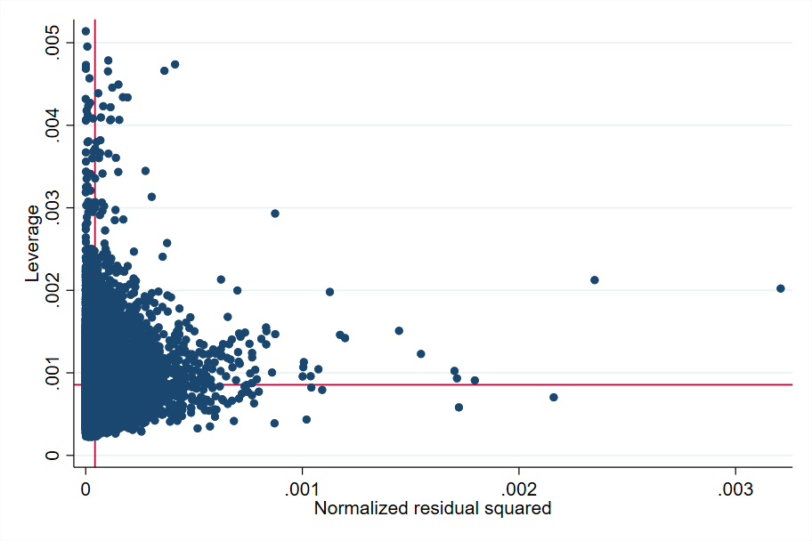
Fig. 6.1 Squared normalized residual vs leverage#
Source: own elaboration from code in Appendix Section 6.4.2. The red lines are references to the mean leverage on the Y axis and the mean squared normalized residual on the X axis. Observations that are far away from these reference points should be inspected more closely.
// Graphic method < after >

    reg y $postvif [aw=Whh] if nogo==0

    // residuals vs fitted vals
    rvfplot , yline(0)  `graphs'

    graph export "$figs\rvfplot_2_after.png", as(png) replace


    // normalized residual squared vs leverage
    lvr2plot ,        `graphs'

    graph export "$figs\lvr2plot_after.png", as(png) replace
6.3.3. Residual analysis#
Most techniques for residual analysis rely on visual inspection of the graphed residuals. Residuals should be checked for linearity, normality, and constant variance in case homoskedasticity is assumed.
6.3.3.1. Linearity#
The nested-error model used in SAE (Equation (6.1)) assumes that the outcome variable \(y\) is a linear function of the covariates.10 If a single covariate is used, a scatter plot of the residual versus the covariate is enough to see if a linear relationship exists. When several covariates are used, checking for linearity is somewhat more complex.
To assess linearity in a simple regression, use scatter to produce a plot of \(y\) versus \(x\), lfit to fit a regression line, and lowess to show a smoothed fit.
. reg depvar indepvar
. twoway (scatter depvar indepvar)(lfit depvar indepvar)(lowess depvar indepvar)
For multiple regression:
. reg depvar indepvars
. predict r, residual
. scatter r indepvar1
. scatter r indepvar2
Other checks for non-linearity include acprlot and cprplot, which produce graphs of an augmented component-plus-residual plot and a residual plot, respectively.
. reg depvar indepvars
. acprplot indepvar1, lowess lsopts(bwidth(1))
. acprplot indepvar2, lowess lsopts(bwidth(1))
When a clear non-linear pattern is observed, transformations of the independent variable might help.
. graph matrix depvar indepvars, half
. kdensity indepvar, normal
. gen logvar=log(indepvar)
. kdensity logvar, normal
6.3.3.2. Tests for normality of residuals and random effects#
Model errors and random effects are assumed to be normally distributed under the nested-error model used for SAE. Deviations from normality may lead to considerable bias in the final small area estimates. Scatter plots of residuals against fitted values and normal Q-Q plots of residuals provide a natural way to identify outliers or influential observations that might affect the precision of the estimates. West et al. [2014] mention that the random effects vector is assumed to follow a multivariate normal distribution. Thus, the information from the observations sharing the same random effect is used to predict (instead of estimating) the values of that random effect in the model.
The usual predictors of the random effects under linear mixed models are known as Empirical Best Linear Unbiased Predictors (EBLUPs), since they are the most precise linear unbiased predictors. They use the weighted least squares estimates of \(\beta\), and the variance parameters are replaced by suitable estimates (Robinson and others [1991]). Rao and Molina [2015] provide a comprehensive formal derivation of the EBLUPs, and applications beyond small area estimation can be found in West et al. [2014].
The xtmixed or mixed command may be used to check the validity of a linear mixed model in Stata. Deviations from normality can be observed in a normal Q-Q plot of residuals (Fig. 6.2), which displays sample quantiles of unit-level residuals against the theoretical quantiles of a normal distribution plot:
mixed depvar indepvars || area:, reml
predict res, residual
qnorm res
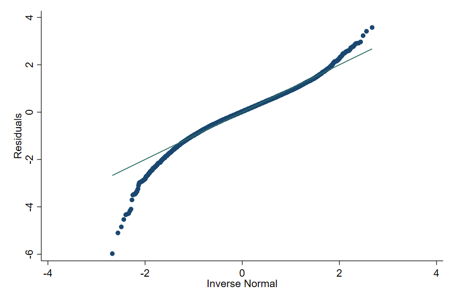
Fig. 6.2 Sample quantiles of residuals against theoretical quantiles of a Normal distribution#
Source: own elaboration from code in Appendix Section 6.4.2. Deviations from normality can be observed in the figure particularly at the bottom. Marhuenda et al. [2017] notes that, in applications using real data, the exact fit to a distribution is hardly met; it is recommended that practitioners apply several transformations to the dependent variable and select the one that provides the best approximation to the nested-error model’s assumptions.
It is also important to check the assumptions regarding the distribution of the random effects. This may be done after fitting the linear mixed model and obtaining the predicted random effects (Fig. 6.3):
predict eta, reffects
bysort area: gen first = _n
qnorm eta if first==1
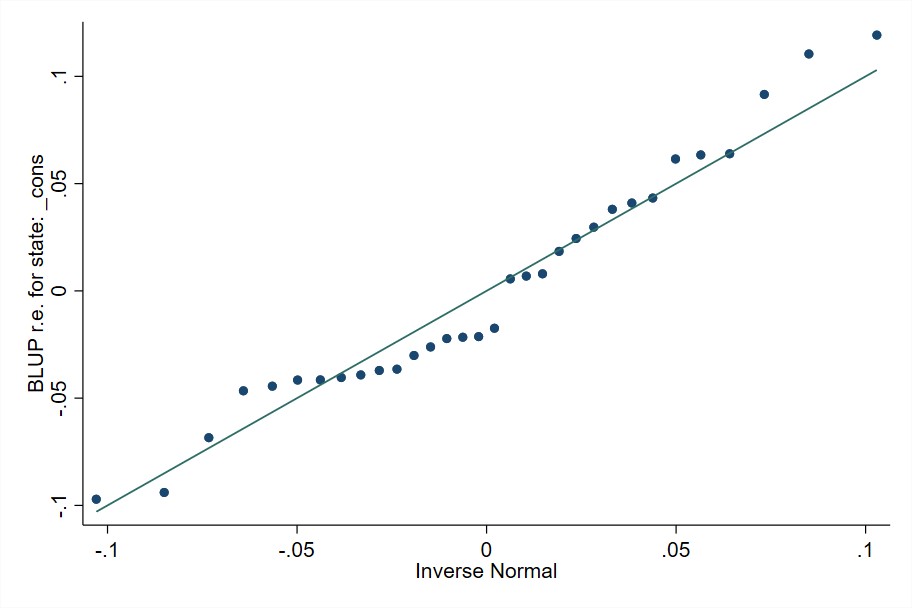
Fig. 6.3 Sample quantiles of predicted random effects against theoretical quantiles of a Normal distribution#
Source: own elaboration.
The plots of empirical quantiles compared to theoretical quantiles of the normal distribution (normal Q-Q plots) are helpful to detect deviations from normality. Transformations of the dependent variable are often taken to ensure that empirical quantiles are better aligned to the theoretical ones. As Marhuenda et al. [2017] note, in real life applications, the exact fit to a distribution is hardly met.
6.4. Appendix#
6.4.1. Useful definitions and concepts#
Definitions are based on Molina and Marhuenda [2015], Ghosh and Rao [1994], Rao and Molina [2015], and Cochran [2007].
Small area: a domain (area) is regarded as small if the domain-specific sample size is not large enough to support direct estimates of adequate precision. That is to say, a small area is any domain of interest for which direct estimates of adequate precision cannot be produced.
Large area: an area or domain where a direct estimate of the parameter of interest for the area has a sufficiently large sample to yield estimates with the desired precision.
Domain: domain may be defined by geographic delimitation/territories (e.g., state, county, school district, health service area), socio-demographic groups, or both (e.g., specific age-sex-race group within a large geographic area) or even other types of sub-populations (e.g., set of firms belonging to a census division by industry group).
Direct (domain) estimators: estimators based only on the domain-specific sample area. These estimators are typically design-unbiased but tend to have low precision in small areas.
Indirect (domain) estimators: estimator that uses information from other areas, under the assumption that there exists some homogeneity relationship between them.
Target parameter: indicator to be estimated. Some examples are population mean, proportion, and rate.
Efficiency/precision: 1/variance when an estimator is unbiased; 1/MSE otherwise.
Sampling error: error from using a sample from the population rather than the whole population.
For a better understanding of statistical inference, the following concepts/definitions are necessary. Definitions and observations are from Molina and García-Portugues [2021] and Rao and Molina [2015]. Note that, when dealing with SAE, the bias for each area \(c=1,\ldots,C\) is of interest, not the average bias over all the areas.
Unbiased estimator: if an estimator’s bias is equal to zero for all the parameter values. If the expected value of the estimator is equal to the parameter. The estimator \(\hat{\vartheta}_{c}\) of parameter \(\vartheta_{c}\) is unbiased if and only if \(E(\hat{\vartheta}_{c}-\vartheta_{c})=0\)
Estimation error: the estimation error \(\hat{\vartheta}_{c}-\vartheta_{c}\) is typically different from zero even if the estimator is unbiased. The bias is the mean estimation error: \(Bias(\hat{\vartheta}_{c})=E(\hat{\vartheta}_{c}-\vartheta_{c})\).
Mean squared (estimation) error (MSE): is also called mean squared prediction error (MSPE) or prediction mean squared error (PMSE). \(MSE(\hat{\vartheta}_{c})=E[(\hat{\vartheta}_{c}-\vartheta_{c})^{2}]\).
Standard error (SE) of \(\hat{\vartheta}_{c}\): is the standard deviation of the sampling distribution of \(\hat{\vartheta}_{c}.\)
Coefficient of variation (CV) of \(\vartheta\): \(cv(\hat{\vartheta})=s(\hat{\vartheta})/\vartheta\) is the associated standard error of the estimate over the true value of \(\vartheta\). It is also known as the relative standard deviation (RSD). The estimated CV is then \(\hat{cv}(\hat{\vartheta})=s(\hat{\vartheta})/\hat{\vartheta}\).
Consistency: when increasing the sample size \(n\), the probability that the estimator differs from the true value \(\vartheta_{c}\) by more than \(\varepsilon\) vanishes for every \(\varepsilon>0\).
6.4.2. Regression diagnostics do-file#
The following Stata do-file provides an example of how regression diagnostics are often incorporated in the model selection process for small area estimation. Note that the checks are not exhaustive and only serve as a guide for the practitioner.
clear all
set more off
/*===============================================================================
Do-file prepared for SAE Guidelines
- Regression Diagnostics
- authors Paul Corral, Minh Nguyen & Sandra Segovia
*==============================================================================*/

global main       "C:\Users\\`c(username)'\OneDrive\SAE Guidelines 2021"
global section    "$main\4_Model_selection"

global data      "$section\1_data"
global dofile    "$section\2_dofiles"
global figs      "$section\3_figures"

local survey       "$data\survey_public.dta"
*local census      "$main\3_Unit_level\1_data\census_public.dta"

//global with candidate variables.
global myvar rural  lnhhsize age_hh male_hh  piped_water no_piped_water ///
no_sewage sewage_pub sewage_priv electricity telephone cellphone internet ///
computer washmachine fridge television share_under15 share_elderly ///
share_adult max_tertiary max_secondary HID_* mun_* state_*


version 15
set seed 648743

local graphs graphregion(color(white)) xsize(9) ysize(6) msize(small)
*===============================================================================
// End of preamble
*===============================================================================

// First part is just as the model selection dofile

// Load in survey data
use "`survey'", clear

	//Remove small incomes affecting model
	drop if e_y<1

    // Kernel density plot  for e_y with a normal density overlaid
    kdensity e_y, normal `graphs'

    graph export "$figs\kdensity_e_y.png", as(png) replace

	//Log shift transformation to approximate normality
	lnskew0 double bcy = exp(lny)

    // Kernel density plot  for lnywith a normal density overlaid
    kdensity lny, normal `graphs'

    graph export "$figs\kdensity_lny.png", as(png) replace

    // Kernel density plot  for bcy with a normal density overlaid
    kdensity bcy, normal `graphs'

    graph export "$figs\kdensity_bcy.png", as(png) replace

    // removes skeweness from distribution
    sum e_y, d
	sum lny, d
	sum bcy, d

	// Data has already been cleaned and prepared. Data preparation and the creation
	// of eligible covariates is of extreme importance.
	// In this instance, we skip these comparison steps because the sample is
	// literally a subsample of the census.
	codebook HID //10 digits, every single one
	codebook HID_mun //7 digits every single one

	//We rename HID_mun
	rename HID_mun MUN
	//Drop automobile, it is missing
	drop *automobile* //all these are missing

	//Check to see if lassoregress is installed, if not install
	cap which lassoregress
	if (_rc) ssc install elasticregress

	//Model selection - with Lasso
	gen lnhhsize = ln(hhsize)
	lassoregress bcy  $myvar [aw=Whh], lambda1se epsilon(1e-10) numfolds(10)
	local hhvars = e(varlist_nonzero)
	global postlasso  `hhvars'

	//Try Henderson III GLS
	sae model h3 bcy $postlasso [aw=Whh], area(MUN)

	//Rename HID_mun
	rename MUN HID_mun

	//Loop designed to remove non-significant covariates sequentially
	forval z= 0.5(-0.05)0.05{
		qui:sae model h3 bcy `hhvars' [aw=Whh], area(HID_mun)
		mata: bb=st_matrix("e(b_gls)")
		mata: se=sqrt(diagonal(st_matrix("e(V_gls)")))
		mata: zvals = bb':/se
		mata: st_matrix("min",min(abs(zvals)))
		local zv = (-min[1,1])
		if (2*normal(`zv')<`z') exit

		foreach x of varlist `hhvars'{
			local hhvars1
			qui: sae model h3 bcy `hhvars' [aw=Whh], area(HID_mun)
			qui: test `x'
			if (r(p)>`z'){
				local hhvars1
				foreach yy of local hhvars{
					if ("`yy'"=="`x'") dis ""
					else local hhvars1 `hhvars1' `yy'
				}
			}
			else local hhvars1 `hhvars'
			local hhvars `hhvars1'
		}
	}

	global postsign `hhvars'


*===============================================================================
// Regression diagnostics
*===============================================================================

/*This is not a complete diagnostic; it is just a preview, steps & repetitions
depend on the underlying model. Check all vars, check different transformations,
do not forget a model for heteroskedasticity (alpha model) if needed */

rename bcy y

*===============================================================================
// Collinearity
*===============================================================================

reg y $postsign [aw=Whh],r

    //Check for multicollinearity, and remove highly collinear (VIF>3)
	cap drop touse 	            //remove vector if it is present to avoid error in next step
	gen touse = e(sample) 		//Indicates the observations used
	estat vif 				    //Variance inflation factor
	local hhvars $postsign

    //Remove covariates with VIF greater than 3
	mata: ds = _f_stepvif("`hhvars'","Whh",3,"touse")
	global postvif `vifvar'

	//VIF check
	reg y $postvif [aw=Whh], r
	vif

    // For ilustration
    // Henderson III GLS - model post removal of non-significant
    sae model h3 y $postsign [aw=Whh], area(HID_mun)

    // Henderson III GLS - model post removal of non-significant
	sae model h3 y $postvif [aw=Whh], area(HID_mun)

*===============================================================================
// Residual Analysis
*===============================================================================

// Linearity

    reg y $postsign, r

    // Augmented component-plus-residual plot; works better than the
    // component-plus-residual plot for identifying nonlinearities in the data.
    acprplot age_hh, lowess lsopts(bwidth(1)) `graphs'

    graph export "$figs\acprplot_age_hh.png", as(png) replace

    // Kernel density plot  for log_age_hh with a normal density overlaid
    kdensity age_hh, normal `graphs'

    graph export "$figs\kdensity_age_hh.png", as(png) replace

    // log transformation
    gen log_age_hh =log(age_hh)

    // Kernel density plot  for log_age_hh with a normal density overlaid
    kdensity log_age_hh, normal `graphs'

    graph export "$figs\kdensity_log_age_hh.png", as(png) replace


// Normality

    reg y $postvif [aw=Whh],r
    predict resid, resid

    // Kernel density plot  for residuals with a normal density overlaid
    kdensity resid, normal `graphs'

    graph export "$figs\kdensity_resid.png", as(png) replace

    // Standardized normal probability
    pnorm resid , `graphs'

    graph export "$figs\pnorm.png", as(png) replace

    // Quantiles of a variable against the quantiles of a normal distribution
    qnorm resid , `graphs'

    graph export "$figs\qnorm.png", as(png) replace

    // Numerical Test:  Shapiro-Wilk W test for normal data
    swilk resid


// Heteroscedasticity

    reg y $postvif

    // Residuals vs fitted values with a reference line at y=0
    rvfplot , yline(0)  `graphs'

    graph export "$figs\rvfplot_1.png", as(png) replace

    // Cameron & Trivedi's decomposition of IM-test / White test
    estat imtest

    // Breusch-Pagan / Cook-Weisberg test for heteroskedasticity
    estat hettest


*===============================================================================
// Influence Analysis
*===============================================================================

// Graphic method < before >

    reg y $postvif [aw=Whh]

    // residuals vs fitted vals
    rvfplot , yline(0)  `graphs'

    graph export "$figs\rvfplot_2.png", as(png) replace


    // normalized residual squared vs leverage
    lvr2plot ,  `graphs'

    graph export "$figs\lvr2plot.png", as(png) replace


// Numerical method


// Step 1

    reg y $postvif

    // After regression without weights...

    // Calculate measures to identify influential observations
	predict cdist, cooksd      // calculates the Cook's D influence statistic
	predict rstud, rstudent    // calculates the Studentized (jackknifed) residuals

// Step 2

    reg y $postvif [aw=Whh]

    // Predict leverage and residuals
	predict lev, leverage  // calculates the diagonal elements of the
                           // projection ("hat") matrix
	predict r, resid       // calculates the residuals

    // Save useful locals
    local myN=e(N)              // # observations
	local myK=e(rank)           // rank or k
    local KK =e(df_m)           // degrees of freedom (k-1)

    sum cdist, d
    * return list
	local max = r(max)          // max value
	local p99 = r(p99)		    // percentile 99

 // Step 3

    // For ilustration...
    // We have influential data points...
    reg lny $postvif if cdist<4/`myN' [aw=Whh]
    reg lny $postvif if cdist<`p99'   [aw=Whh]
	reg lny $postvif if cdist<`max'   [aw=Whh]

    // Identified influential / outliers observations
    gen nogo = abs(rstud)>2 & cdist>4/`myN' & lev>(2*`myK'+2)/`myN'

    count if nogo==1        // these are the obs that we want to eliminate


// Graphic method < after >

    reg y $postvif [aw=Whh] if nogo==0

    // residuals vs fitted vals
    rvfplot , yline(0)  `graphs'

    graph export "$figs\rvfplot_2_after.png", as(png) replace


    // normalized residual squared vs leverage
    lvr2plot ,        `graphs'

    graph export "$figs\lvr2plot_after.png", as(png) replace


*===============================================================================
// Model Specification tests
*===============================================================================

   reg y $postvif

// Wald test for ommited vars < will compare with previous regression>
   boxcox y $postvif, nolog // Box - Cox model


// Functional form of the conditional mean
    reg y $postvif

    estat ovtest // performs regression specification error test (RESET) for omitted variables

    linktest //performs a link test for model specification

// Omnibus tests + Heteroscedasticity tests
    reg y $postvif

    estat imtest   // Cameron & Trivedi's decomposition of IM-test / White test

    estat hettest // Breusch-Pagan / Cook-Weisberg test for Heteroscedasticity


*===============================================================================
// Diagnostics for random effects
*===============================================================================

// Multilevel mixed-effects linear regression
    mixed y $postvif || state:, reml

    predict res, residual

    predict eta, reffects

    bysort state: gen first=_n

    // For state == 1
    qnorm eta if first==1 , `graphs'

    graph export "$figs\qnorm_mixed_1.png", as(png) replace


// Quantiles of a variable against the quantiles of a normal distribution
    qnorm res , `graphs'

    graph export "$figs\qnorm_mixed.png", as(png) replace
Note
And for the figures
set more off
clear all

*===============================================================================
//Macros for inputs to the simulation
*===============================================================================

// Replication of Molina and Rao's 2010 simulation - SAE Guidelines
global main    "C:\Users\\`c(username)'\OneDrive\WPS_2020\"
global dpath   "$main\1.data"
global simdata "$dpath\"
global thedo   "$main\2.dofiles\Model sim\"
global XL 	   "$main\SAE result summary.xlsx"

	local direct           Direct
	local h3area		   Unit-Context CEB
	local true             True
	local ellold           ELL - with context (collapsed)
	local h3eb             CensusEB
	local h3ebc            CensusEB - with context (collapsed)
	local ell			   ELL - with context (New Sim)
	local twofold          Twofold nested error CEB
	local twofoldA         U-C twofold nested error CEB


	local direct_s           ms(+)
	local h3area_s		     mcolor(black) msize(small) msymbol(O)
	local ellold_s           mcolor(gray) msize(small) msymbol(X)
	local h3eb_s             mcolor(green) msize(small) msymbol(t)
	local h3ebc_s            mcolor(green) msize(small) msymbol(Sh)
	//local ell_s				 mcolor(gray)  msiz(vsmall) msymbol(Th)
	local twofold_s            mcolor(red)  msiz(small) msymbol(Oh)
	local twofoldA_s           mcolor(blue)  msiz(vsmall) msymbol(D)

// Replication of Molina and Rao's 2010 simulation - SAE Guidelines
local indis fgt0 fgt1 fgt2 Mean
local simres1 h3ebc h3eb direct h3area ellold ell twofold twofoldA
local simres2 h3ebc h3eb direct h3area ellold ell twofold twofoldA
local simres3 h3ebc h3eb direct h3area ellold ell twofold twofoldA
local simres4 h3ebc h3eb direct h3area ellold ell twofold twofoldA

*===============================================================================
// Figures for models
*===============================================================================


foreach i in Mean fgt0 fgt1 fgt2{
	foreach sim in 1 2 3 4{
		use "$simdata\accumulate_results.dta", clear
		lab var area "Area"

		keep if simulation==`sim'
		replace `i'_bias=`i'_bias*100
		replace `i'_mse=`i'_mse*10000
		local forlab = upper("`i'")
		lab var `i'_bias "Bias `forlab' (x100)"
		lab var `i'_mse "MSE `forlab' (x10000)"

		foreach b in bias mse{
			twoway scatter `i'_`b' area if method=="direct", sort `direct_s' || ///
			scatter `i'_`b' area if method=="twofold", sort `twofold_s' || ///
			scatter `i'_`b' area if method=="h3eb", sort `h3eb_s' || ///
			scatter `i'_`b' area if method=="h3ebc", sort `h3ebc_s' || ///
			scatter `i'_`b' area if method=="ellold", sort `ellold_s' || ///
			scatter `i'_`b' area if method=="h3area", sort `h3area_s' || ///
			scatter `i'_`b' area if method=="twofoldA", sort `twofoldA_s' ||, ///
			legend(order(1 "`direct'" 2 "`twofold'" 3 "`h3eb'" 4 "`h3ebc'" 5 "`ell'" 6 "`h3area'" 7 "`twofoldA'")) graphregion(color(white))

			graph export "$main/4.figures//`b'_sim`sim'_`i'.png", replace as(png)
		} // End bias/mse
	} //End sim
} //End measures
		sss
//Question, how does the estimated MSE look like when collapsing H3EB to the next level?
use "$simdata\accumulate_results.dta", clear

foreach x of varlist fgt0_ms* fgt1_ms* fgt2_ms* Mean_ms*{
	replace `x' = sqrt(`x')
}
foreach x of varlist fgt0_bias* fgt1_bias* fgt2_bias* Mean_bias*{
	gen `x'_abs = abs(`x')
}


sp_groupfunction, mean( fgt0_bias_rel_abs fgt1_bias_rel_abs fgt2_bias_rel_abs fgt0_mse_rel fgt1_mse_rel fgt2_mse_rel Mean_bias_rel_abs Mean_mse_rel  fgt0_bias_abs fgt1_bias_abs fgt2_bias_abs Mean_bias_abs *_mse) by(method sim)


gen concat = method+"_"+variable+"_"+string(sim)
order concat, first

export excel using "$XL", sheet(result) sheetreplace first(var)
6.5. References#
- CT05
A Colin Cameron and Pravin K Trivedi. Microeconometrics: methods and applications. Cambridge university press, 2005. ISBN 978-0-521-84805-3.
- Coc07
William G Cochran. Sampling techniques. John Wiley & Sons, 2007.
- Coo77
R Dennis Cook. Detection of influential observation in linear regression. Technometrics, 19(1):15–18, 1977.
- CHMM21
Paul Corral, Kristen Himelein, Kevin McGee, and Isabel Molina. A map of the poor or a poor map? Mathematics, 2021. URL: https://www.mdpi.com/2227-7390/9/21/2780, doi:10.3390/math9212780.
- CMN21(1,2)
Paul Corral, Isabel Molina, and Minh Cong Nguyen. Pull your small area estimates up by the bootstraps. Journal of Statistical Computation and Simulation, 91(16):3304–3357, 2021. URL: https://www.tandfonline.com/doi/abs/10.1080/00949655.2021.1926460, doi:10.1080/00949655.2021.1926460.
- ELL03(1,2)
Chris Elbers, Jean O Lanjouw, and Peter Lanjouw. Micro–level estimation of poverty and inequality. Econometrica, 71(1):355–364, 2003.
- ELL02
Chris Elbers, Jean Olson Lanjouw, and Peter Lanjouw. Micro-level estimation of welfare. World Bank Policy Research Working Paper, 2002.
- GR94
Malay Ghosh and JNK Rao. Small area estimation: an appraisal. Statistical science, 9(1):55–76, 1994.
- JWHT13(1,2,3)
Gareth James, Daniela Witten, Trevor Hastie, and Robert Tibshirani. An introduction to statistical learning. Volume 112. Springer, 2013. ISBN 978-1-0716-1418-1. URL: https://link.springer.com/book/10.1007/978-1-0716-1418-1?noAccess=true.
- LS15
Partha Lahiri and Jiraphan Suntornchost. Variable selection for linear mixed models with applications in small area estimation. Sankhya B, 77(2):312–320, 2015.
- MMMR17(1,2)
Yolanda Marhuenda, Isabel Molina, Domingo Morales, and JNK Rao. Poverty mapping in small areas under a twofold nested error regression model. Journal of the Royal Statistical Society: Series A (Statistics in Society), 180(4):1111–1136, 2017. doi:10.1111/rssa.12306.
- MGarciaP21
Isabel Molina and Eduardo García-Portugues. A First Course on Statistical Inference. Bookdown.org, 2021. Accessed: 2010-06-22. URL: https://bookdown.org/egarpor/inference/.
- MM15
Isabel Molina and Yolanda Marhuenda. Sae: an R package for small area estimation. The R Journal, 7(1):81–98, 2015.
- MR10
Isabel Molina and JNK Rao. Small area estimation of poverty indicators. Canadian Journal of Statistics, 38(3):369–385, 2010.
- MohringSC13(1,2)
Katja Möhring and Alexander Schmidt-Catran. Mlt: stata module to provide multilevel tools. 2013. URL: https://econpapers.repec.org/software/bocbocode/s457577.htm.
- Pfe13
Danny Pfeffermann. New important developments in small area estimation. Statistical Science, 28(1):40–68, 2013.
- RM15(1,2,3,4,5,6,7)
JNK Rao and Isabel Molina. Small Area Estimation. John Wiley & Sons, 2nd edition, 2015.
- R+91
George K Robinson and others. That blup is a good thing: the estimation of random effects. Statistical science, 6(1):15–32, 1991.
- TZL+18
Nikos Tzavidis, Li-Chun Zhang, Angela Luna, Timo Schmid, and Natalia Rojas-Perilla. From start to finish: a framework for the production of small area official statistics. Journal of the Royal Statistical Society: Series A (Statistics in Society), 181(4):927–979, 2018.
- WWG14(1,2)
Brady T West, Kathleen B Welch, and Andrzej T Galecki. Linear mixed models: a practical guide using statistical software. Chapman and Hall/CRC, 2nd edition, 2014. URL: https://www.taylorfrancis.com/books/mono/10.1201/b17198/linear-mixed-models-brady-west-kathleen-welch-andrzej-galecki, doi:10.1201/b17198.
6.6. Notes#
- 1
Except for the gradient boosting application shown.
- 2
The authors define the approximation error as the difference between standard variable selection criterion and the ideal variable selection criterion, where it is assumed that the direct estimates are not measured with noise.
- 3
See Corral et al. [2021] for a detailed discussion on the previous ELL bootstrap. Also see Elbers et al. [2002] for the sources of noise in their algorithm.
- 4
LMM are an extension of general linear models which include both fixed and random effects.
- 5
These assumptions are similar to the ones of a classic linear regression, but adding those for the random effects inclusion.
- 6
Many of the commands provided in the following subsections can be easily reviewed by typing
help regress postestimationin Stata’s command window.- 7
The Mata function is included in Stata’s
saepackage.- 8
The specific threshold value is up to the practitioner, although it is not recommended to use thresholds above 10.
- 9
https://www.stata.com/meeting/germany12/abstracts/desug12_moehring.pdf
- 10
Much of the information in this section is borrowed from ; https://stats.idre.ucla.edu/stata/webbooks/reg/chapter2/stata-webbooksregressionwith-statachapter-2-regression-diagnostics/