Unit-level Models for Small Area Estimation
Contents
4. Unit-level Models for Small Area Estimation#
This chapter focuses on unit-level models for small area estimation of poverty, which typically rely on estimating the distribution of the household’s welfare, given a set of auxiliary variables or correlates.1 The methods presented in this chapter use model-based techniques that “borrow strength” from other areas by using a larger data set with auxiliary information – usually the population census. The resulting indirect estimators sacrifice design bias, but often yield more precise estimates in terms of mean-squared errors (MSE). In software implementations of the method described in this chapter, model parameters are used to simulate multiple welfare vectors from the fitted distribution for all households in the census. This is done because the census often lacks a welfare measure for poverty measurement (Elbers et al. [2007]). From the simulated census vectors, it is possible to obtain poverty rates or any other welfare indicator, for every area, including the non-sampled ones. This chapter serves as a guide for the production of unit-level small area estimates of poverty indicators, focusing on two of the most popular approaches – the one proposed by Elbers, Lanjouw, and Lanjouw (Elbers et al. [2003], ELL), and the Empirical Best (EB) approach by Molina and Rao (Molina and Rao [2010], MR).2 It presents evidence on certain aspects of SAE and recommendations on what may be the preferred approach in some scenarios and offers advice for aspects where perhaps more research is needed.
The chapter begins by presenting some of the prerequisites that should be satisfied before commencing a SAE exercise. It provides insights that may help practitioners choose a unit-level SAE method that is adequate for their needs. It then presents considerations that practitioners may keep in mind when conducting SAE, such as data transformation and why ELL has fallen out of favor with many practitioners. Additionally, it presents the usual steps towards selecting a model and the production of small area estimates. The sections rely on real world and simulated data, and offer codes which readers may use to replicate some of the analysis; in other instances it pulls evidence from recent research.3
4.1. Preparing for Unit-Level Small Area Estimation#
The basic ingredients for model-based unit-level small area estimation for poverty are a contemporaneous survey and census – ideally from the same year. Small area estimates rely on household-level data to obtain the conditional distribution of welfare given the observed correlates. This information is then used to generate welfare for all the census units. Thus, if characteristics in the two datasets differ considerably, or if the structure of the conditional distribution has changed between the two data sources, then the estimates could be biased and of little use.
Obtaining a pool of candidate variables for the analysis requires a thorough review of the survey and census data to ensure comparability. In the census and survey questionnaires, questions should be asked in a similarly, ideally worded in the same manner. Checks should then be conducted on the survey weights to understand how these are constructed. For example, in some countries where there is heavy migratory work, household expansion factors (usually the number of household members) may be adjusted by the number of days the individual is present in the dwelling. Such adjustments should also be possible in the census data; otherwise, the poverty estimates obtained from SAE methods will not be comparable to those obtained directly from the survey. Even if questions are asked in a similar fashion and weights are replicable, differences may still arise. Teams are strongly recommended to compare the mean and distribution the potential pool of covariates across the survey and the census – including whether it is possible to reproduce the direct estimates of poverty produced by the National Statistical Office. Ideally, the mean and distribution of the covariates should be comparable, at least at the aggregation level at which the survey is designed to be representative.
One of the first decisions that must be made is the level at which estimates must be produced. As noted afterward, this determines the level at which location effects are specified in the model in unit-level models. For reasons that will be apparent in the following sections, the locations in the survey must be matched to the locations in the census. Matching locations will also ensure that when using information from external sources, for example, administrative data or satellite imagery-derived data, these correspond to the correct location. Additionally, the use of hierarchical identifiers for the location variable is recommended (Zhao [2006]). Under Stata’s sae package, these identifiers must be numeric and no longer than 16 digits,4 and should have an equal number of digits for every area. For example, in the hierarchical identifier SSSMMMMPPP, the first 3 digits represent states (S), the next 4 digits represent municipalities (M), and the final 3 digits represent PSUs (P). The use of hierarchical identifiers is necessary for two-fold nested-error models. In the code syntax, the user needs to indicate the number of digits to remove (from the right) to arrive at the larger area’s identifier. For example, to go from PSU to municipality level, it is necessary to remove 3 digits, yielding SSSMMMM.
4.1.1. The Assumed Model#
The model-based small area estimation methods described in this chapter are dependent on an assumed model. The nested-error model used for small area estimation by ELL (Elbers et al. [2003]) and MR ([Molina and Rao, 2010]) was originally proposed by Battese et al. [1988] to produce county-level corn and soybean crop area estimates for the American state of Iowa. For the estimation of poverty and welfare, the ELL and MR methods assume that the transformed welfare \(y_{ch}\) for each household \(h\) within each location \(c\) in the population is linearly related to a \(1\times K\) vector of characteristics (or correlates) \(x_{ch}\) for that household, according to the nested-error model:
where \(\eta_{c}\) and \(e_{ch}\) are respectively location and household-specific idiosyncratic errors, assumed to be independent from each other, following:
where the variances \(\sigma_{\eta}^{2}\) and \(\sigma_{e}^{2}\) are unknown. Here, \(C\) is the number of locations in which the population is divided and \(N_{c}\) is the number of households in location \(c\), for \(c=1,\ldots,C\). Finally, \(\beta\) is the \(K\times1\) vector of regression coefficients.5
One of the main assumptions is that errors are normally distributed. The assumption does not necessarily imply that the transformed welfare (the dependent variable) is normally distributed but instead implies that conditional on the observed characteristics the residuals are normally distributed. Under the assumed model, variation in welfare across the population is determined by three components: the variation in household characteristics, the variation in household-specific unobservables, and the variation in location-specific effects. Within any given area, the welfare distribution is determined by the variation in household specific characteristics and household specific errors.
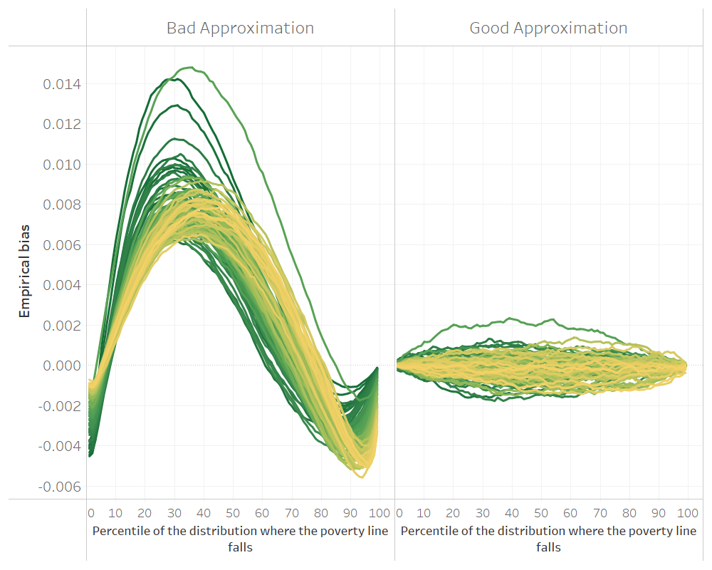
Fig. 4.1 Empirical bias of two different models for unit-level small area estimation#
Source: Simulation based on 1,000 populations generated as described in this Section 5.5.1.1. Each line corresponds to one of the 100 areas of the population. The x-axis represents the percentile on which the poverty line falls on, and the y-axis is the empirical bias. The do-file to replicate these results can be found in Section 5.5.2.
It is important to note that while the method’s goal may be to produce headcount poverty rates or other welfare indicators, these are not explicitly modeled in the sense that the dependent variable is welfare (or transformed welfare) and not the desired indicator (e.g. headcount poverty). The methodology relies on approximating as closely as possible the welfare distribution in each area. A model that approximates the welfare distribution poorly may yield a decent estimate for a given poverty line, yet when judged at a different poverty line the method may completely fail. This can be seen in Fig. 4.1, where the headcount poverty estimates from the model on the left may work relatively well if the poverty threshold were set at the 70th percentile and yield completely biased estimates at most other thresholds. On the other hand, the model on the right approximates the welfare distribution well in all areas and yields poverty estimates with a small bias across all poverty thresholds and areas.
4.2. Conducting Your First SAE Application with a Unit-Level Model#
The focus of this section is on the process of producing small area estimates of monetary indicators using a census and a survey. For the exercise conducted in the following sections it is assumed that the data has already been prepared and all of the checks noted in Section 4.1 have been conducted. The section provides step-by-step processes for producing small area estimates of poverty using census and survey data. It also draws from existing evidence to make recommendations based on current best practices for conducting SAE applications.
4.2.1. Model Choice Considerations#
Ideally, the particular model to be used should be aligned to the specific SAE goals. One of the main considerations regarding the model to be used is the level at which poverty estimates will be reported. This will determine the level at which the random location effect should be specified (see Section 4.4 for details). Specifying the random effects at a lower level of aggregation than the level at which estimation is desired (e.g., for clusters nested within the areas of interest) will lead to noisier estimates (Marhuenda et al. [2017]), albeit with little effect on bias (Corral et al. Corral et al. [2021]). The magnitude by which the MSE of the estimates based on a model with cluster effects instead of area effects will increase depends on the ratio between the variances of the random effects associated to the different locations. If the variance of the random effects of the clusters within areas, \(\sigma_{ac}^{2}\), is larger than that of the area’s random effects, \(\sigma_{a}^{2}\), then the MSE may not increase by much. On the other hand, when the variance of the area’s random effects is larger, the MSE of the estimates based on a model with only cluster effects worsens considerably. Thus, the random location effect should be at the same level for which estimates will be reported (see Fig. 4.2).
Additionally, under the latest edition of the Stata sae package, practitioners can apply two-fold nested-error models (Marhuenda et al. [2017]), besides the traditional one-fold nested-error model. The drawback of the implemented two-fold nested-error model in the Stata sae package is that it does not consider survey weights, nor does it consider heteroskedasticity. The benefit from applying a two-fold nested-error model is that the resulting estimates are optimal at two levels of aggregation, because the MSEs of the estimates at both levels tend to be smaller under the assumed model than when using one-fold nested-error models with only cluster or area effects (see Fig. 4.2).
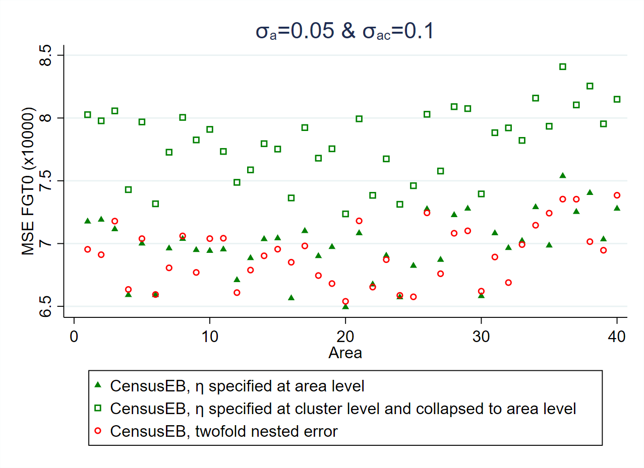
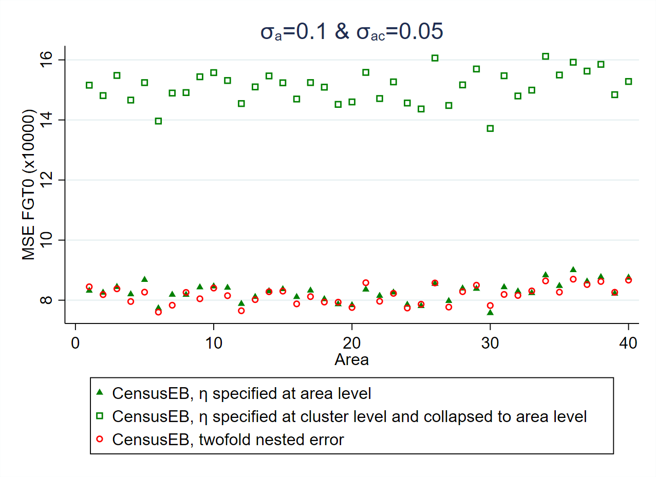
Fig. 4.2 Empirical MSE comparison considering only cluster effects and when aggregating the cluster level results to the area level versus specifying the random effects at the reporting level, area.#
Source: Simulation based on populations generated as described in Corral et al. (Corral et al. [2021]) section 3. Notice how the empirical MSE of CensusEB one-fold nested-error models, where \(\eta\) is specified at the area level, are closely aligned to those under the two-fold nested-error model with cluster and area effects. On the other hand, CensusEB estimators based on one-fold nested-error models, where \(\eta\) is specified at the cluster level, have a considerably larger empirical MSE.
Two model fitting approaches are available under Stata’s sae package: restricted maximum likelihood (REML) and Generalized Least Squares (GLS), where the variance parameters are estimated using Henderson’s method III (Henderson [1953], H3). Both approaches yield similar estimated regression coefficients when heteroskedasticity and survey weights are not considered (Corral et al. [2021] – Figure A4). Given the different available models implemented in Stata’s sae package, it is important to understand which options are available under each fitting method.
Model fit by REML does not incorporate survey weights nor heteroskedasticity. Uses Stata’s
xtmixedcommand in the background to fit the model.6When choosing this fitting method, the one-fold nested-error model considered is the same one used in Molina and Marhuenda’s (Molina and Marhuenda [2015])
saepackage in R. Stata’ssaepackage implements a similar REML fitting approach to Molina and Marhuenda’s Molina and Marhuenda [2015]saeR package.7sae model reml ``depvar indepvars`` [if] [in], area(varname)Beyond the model fitting method, it is also possible to approximate the original Molina and Marhuenda’s Molina and Marhuenda [2015] EB estimates by Monte Carlo simulation (replace
modelbysim) by adding the optionappendsvy.However, the default approach obtains CensusEB8 estimates instead of the original EB ones.Stata’s
saepackage also implements the two-fold nested-error model with cluster effects nested within area effects considered by Marhuenda et al. [2017]. This model is appropriate when point estimates at two different levels of aggregation are desired. Section 4.2.4 presents the hierarchical identifiers needed for specifying two-fold nested-error models.9sae model reml2 ``depvar indepvars`` [if] [in], area(#) subarea(varname)Here the
subareaoption requires an identifier for sub-areas of an equal number of digits for every area. Under theareaoption, the user should specify the number of digits of the hierarchical ID to remove from the right to the left to arrive at an identifier for the areas. These identifiers are commonly referred to as hierarchical identifiers and are explained in Nguyen et al. [2018] and Zhao [2006] in greater detail. Through Monte Carlo simulation (replacemodelbysim) the approach yields CensusEB estimates based on the two-fold nested-error model.
Model fit with GLS, where variance parameters, estimated under Henderson’s method III Henderson [1953], do allow for the inclusion of heteroskedasticity and survey weights according to Van der Weide Van der Weide [2014].10 However, this method has only been implemented for one-fold nested-error models.11
sae model h3 ``depvar indepvars`` [if] [in] [aw], area(varname) [zvar(varnames)yhat(varnames) yhat2(varnames) alfatest(new varname)]The method will obtain CensusEB estimates for areas present in the survey and the census. When weights and heteroskedasticity are not specified, results will be very close to those from
sae model reml(Corral et al. [2021]).The
alfatestoption allows users to obtain the dependent variable for the alpha model, a model for heteroskedasticity introduced in Elbers et al. [2002].12 The resulting dependent variable for the alpha model can facilitate the selection of a suitable model. The covariates for the alpha model are specified underzvarand, when interactions with the main model’s linear fit \(X\hat{\beta}\) are desired, then users may specify covariates under theyhatandyhat2options for the interaction of covariates with \(X\hat{\beta}\) and \((X\hat{\beta})^{2}\), respectively.An updated GLS method with an adaptation of Henderson’s method III Henderson [1953] that incorporates the error decomposition to estimate \(\sigma_{\eta}^{2}\) and \(\sigma_{e}^{2}\) as described in Elbers et al. [2002] and Nguyen et al. [2018] is available.13 When users select this fitting method it is not possible to obtain EB or CensusEB estimates and does not require linking between survey and census areas, and hence not recommended.14 It is still available in Stata’s
saepackage to allow for comparisons and replicability.15sae model elldepvar indepvars`` [if] [in] [aw], area(varname) [zvar(varnames)yhat(varnames) yhat2(varnames) alfatest(new varname)]The
alfatest, zvar, yhat,andyhat2options are similar to those described under H3 fitting method.
The most crucial difference between ELL and EB methods is that ELL estimators are obtained from the distribution of welfare without conditioning on the variable survey sample data, though other differences between the original ELL Elbers et al. [2003] and MR (Molina and Rao [2010]) exist. For example, though the underlying assumed model is the same, different model-fitting approaches are applied between ELL and MR approaches. Noise estimates of the small area estimators are also obtained differently. The implementation of ELL in PovMap draws from the multiple imputation literature, where minimizing the MSE is not the primary goal, while MR’s method relies on the assumed model’s data generating process to estimate the noise of the small area estimators with a parametric bootstrap introduced by González-Manteiga et al. [2008].16
Regardless of the model’s structure (one-fold or two-fold) and the model-fitting approach used (REML or H3 in Stata’s sae package), users are advised to obtain Empirical Best (EB) or CensusEB estimates rather than ELL estimates, because EB will yield more accurate and efficient estimates since EB conditions on the survey sample data and makes more efficient use of the information at hand - see Corral et al. [2021] for a detailed comparison, also see Section 4.4.1.17 The gains from EB can be quite considerable when the assumed model holds (Fig. 4.3, left), but simulations based on real-world data, where the validity of the assumed model is in doubt, also show gains (Fig. 4.3, right).18 Thus, despite ELL being one of the optional approaches in the Stata sae package, it is not recommended because EB estimates will yield more accurate and efficient estimates, see Corral et al. [2021] and Section 4.4.1.19
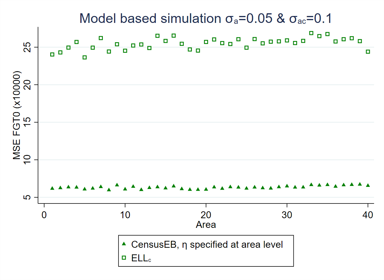
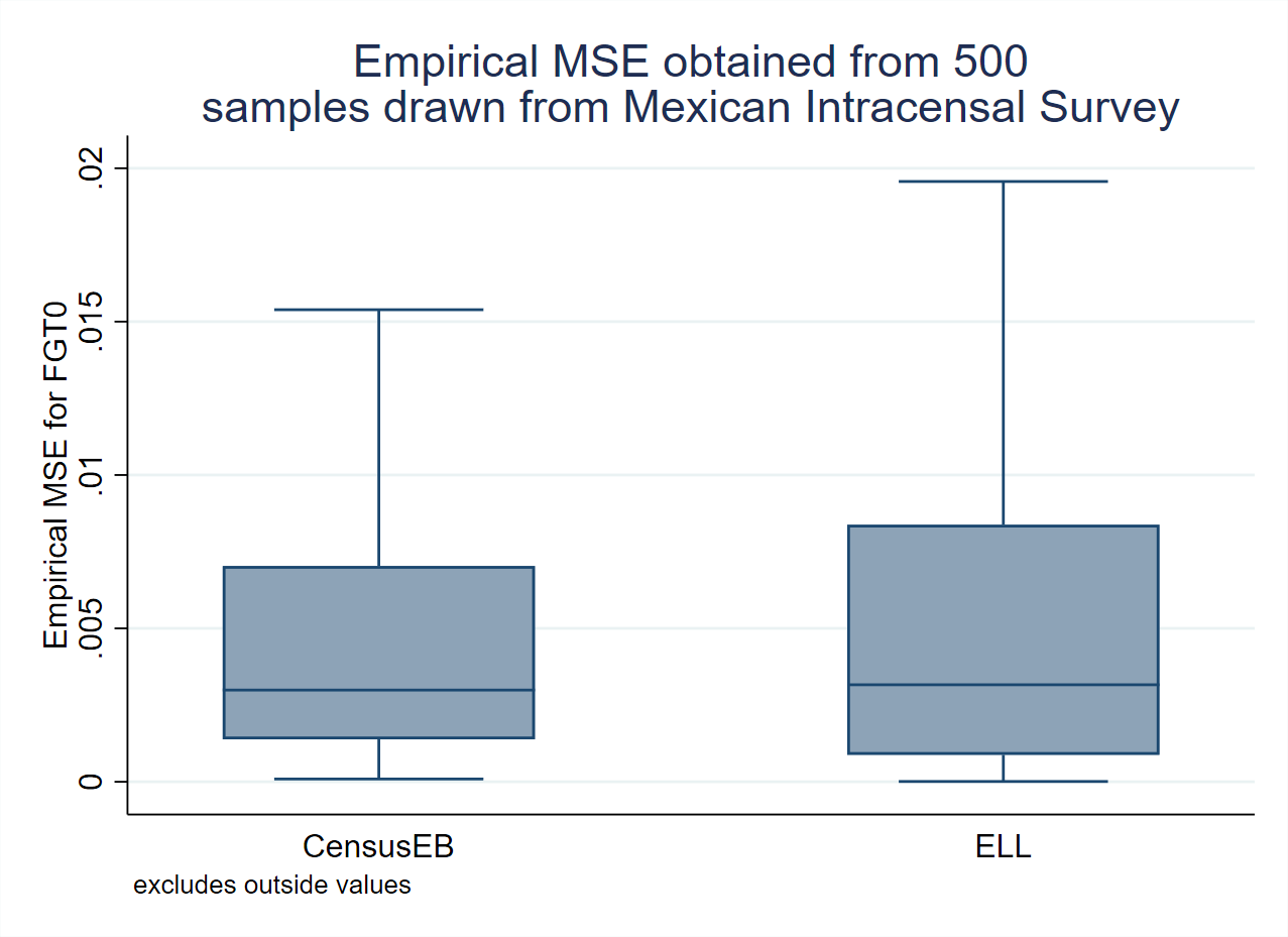
Fig. 4.3 Empirical MSE comparison between ELL and CensusEB#
Source: Simulation based on populations generated as described in Corral et al. [2021], section 3 and 4. The simulations illustrate how the empirical MSE of ELL estimates is considerably larger than that of CensusEB under simulated data (left) and also under real world data (right).
The use of contextual variables in the unit-level model is also recommended as long as their regression coefficients are significant. ELL (Elbers et al. [2002]) noted the importance of explaining the variation in welfare due to location and recommended the inclusion of location means of household-level characteristics, as well as covariates derived from Geographic Information Systems (GIS). Contextual level variables were also noted by Haslett () as being essential in ELL to reduce area-specific bias and standard errors. Since contextual variables can help explain between-area variations, these reduce the portion of unexplained between-area variation and complement household-level information to produce more precise estimates. An example of the value that contextual variables may provide in SAE can be seen in Fig. 4.4, obtained in simulations using real world data. Poverty estimates obtained without contextual variables present more bias and a considerably larger MSE, though specific results will depend on the chosen variables and the data at hand.
As noted, the Stata sae package offers practitioners the option to fit ELL, EB or CensusEB estimates. CensusEB estimates are similar to EB, except that households are not linked across Census and survey data. In practice, the sample size of a given area in the survey is typically much smaller than the actual population size. In these cases, the difference between CensusEB and EB is negligible. In Corral et al. [2021] simulation experiments, where the sample by area is 4 percent of the total population, the difference between EB and CensusEB’s empirical MSE is already indiscernible,
see Fig. 4.5.
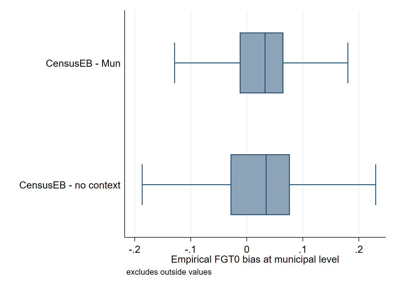
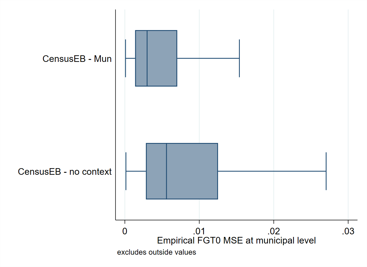
Fig. 4.4 Empirical bias and MSE of Census EB estimators based on a nested-error model with and without contextual variables#
Source: Simulation based on populations generated as described in Corral et al. [2021] section 3 and 4. These design-based simulations provide an example of the possible gains in terms of bias and MSE, obtained from adding contextual variables to the nested-error model.
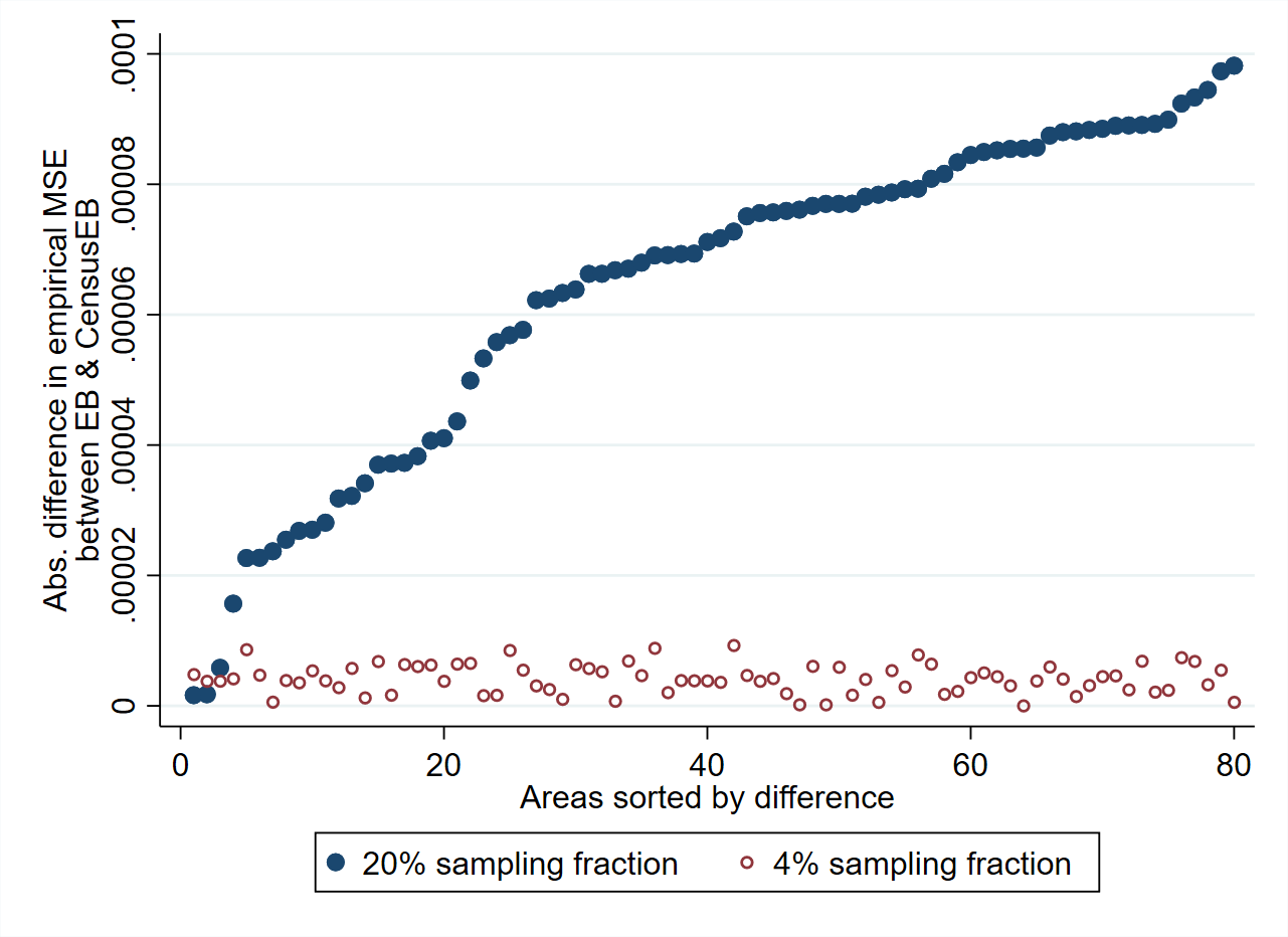
Fig. 4.5 Empirical MSE difference between EB and CensusEB depending on sampling fraction#
Source: Corral et al. [2021]. Figure illustrates that the difference in empirical MSE of CensusEB and EB will be close to zero as the sample fraction of the population decreases.
4.2.2. Data Transformation#
Since the EB method of MR (Molina and Rao [2010]) assumes that the errors are normally distributed, data transformation to get a distribution close to normal can lead to less biased and less noisy estimates (see Rao and Molina [2015]; Rojas-Perilla et al. [2020]; Corral et al. [2021]; and Tzavidis et al. [2018]).20 More generally, variable transformation to make the assumptions underlying the model hold is one of the main aspects of model-based small area estimation (see Technical Annex of this chapter, Section 4.4.1). Specifically, since the SAE models used often assume normality in the errors, the goal in data transformation is to approximate normally distributed residuals.21
Most software packages for small area estimation offer the possibility of data transformation. Perhaps the most popular transformation is the natural logarithm, although it is not always ideal as it can produce left skewed distributions for small values of welfare (see Fig. 4.7). Other options include transformation from the Box-Cox family (Box and Cox [1964]) and the log-shift transformations, which have the advantage that the transformation parameters may be driven by the specific data at hand (Tzavidis et al. [2018]).The Box-Cox family’s transformation parameter, which is the power to be taken, is denoted by \(\lambda\). When \(\lambda=0\), it yields the natural logarithm; otherwise, \(\lambda\) is typically data-driven and chosen to minimize skewness in the dependent variable., which is the power to be taken, is denoted by \(\lambda\). When \(\lambda=0\), it yields the natural logarithm; otherwise, \(\lambda\) is typically data-driven and chosen to minimize skewness in the dependent variable.22 A log-shift transformation adds a positive shift to the observed welfare values before taking the log to avoid the left skewness caused by taking the log of very small welfare values. Other options, such as the ordered quantile normalization (Peterson and Cavanaugh [2019]), may generate reliable estimates of headcount poverty, but these transformations are not reversible and therefore they cannot be used to obtain other indicators such as mean welfare, poverty gap, poverty severity among others (Masaki et al. [2020]; Corral et al. [2021]), limiting their applicability. Regardless of the transformation chosen, it is always recommended to check the residuals to determine if these follow the underlying model assumptions.
When working with real-world data, assumptions are often only approximately met (Marhuenda et al. [2017]) and effort must be made to find one that approximates the normal distribution best. In simulation studies that seek to validate small area estimation methods based on actual data, data-driven transformations may reduce bias and the noise due to departures from normality (see Corral et al. [2021] and Tzavidis et al. [2018] among others). Using the Mexican Intercensal survey of 2015 as a 3.9 million household census data, Corral et al. [2021] note that the gains from a transformation of the dependent variable that minimizes skewness can be quite considerable. In the validation exercises conducted in that paper, bias and MSEs, are considerably reduced when using a Box-Cox or a log-shift transformation (see Fig. 4.6).
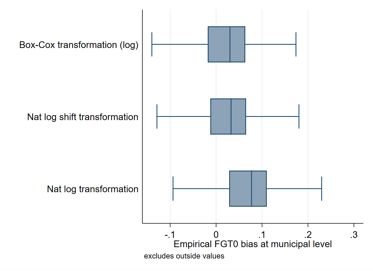
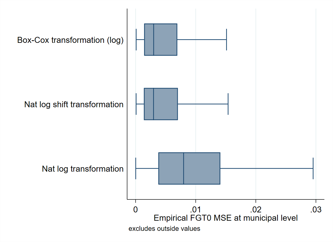
Fig. 4.6 Empirical Bias and MSE for CensusEB FGT0 estimates under different transformations#
Source: Based on samples generated as described in Corral et al. [2021] section 4. The figure illustrates the potential gains from a correct data transformation. Taking the natural logarithm of the dependent variable in this case is not enough and can lead to considerable deviations from normality and thus may yield larger empirical MSEs and biased predictors.
Implementation of a suitable data transformation in Stata is straightforward, since Stata offers commands for the Box-Cox and the zero-skewness log (log-shift) transformation.23 The Stata sae package (Nguyen et al. [2018]) also includes these transformations, in addition to the natural logarithm, as options and will apply the transformation for the model. The package will also reverse the transformation to calculate the indicators of interest in each Monte Carlo simulation. Prior to estimating the indicators, practitioners may wish to do model selection (e.g., by lasso or stepwise regression) using an already transformed dependent variable. Once the transformed dependent variable is obtained, practitioners can then conduct histograms and visually inspect the shape of the distribution of the dependent variable (see Fig. 4.7).
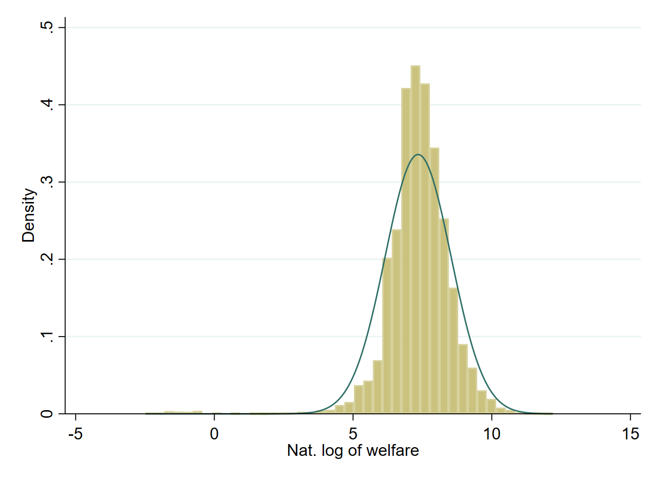
Fig. 4.7 Natural logarithm of welfare#
Source: Corral et al. [2021] . The figure illustrates how, in this case, taking the natural logarithm of welfare leaves a left skewed distribution which may yield biased and noisier estimators.
Once a satisfactory transformation is obtained, the process of model selection of the covariates can occur. The model selection process consists of selecting the response variable and the most powerful set of covariates such that the assumptions underlying the chosen SAE method hold – primarily linearity and normality of the residuals. The consequences of deviations from the underlying model’s assumptions could lead to invalid inferences (Rao and Molina [2015]) or not too noisy but biased estimates (Banerjee et al. [2006]). The model selection procedure is further explored in Chapter 6: Model Diagnostics in Section 6.2.
4.2.3. The Alpha Model#
The alpha model proposed by ELL (Elbers et al. [2002]) is a preliminary model for the variance of the idiosyncratic errors used for heteroskedasticity that resembles the one presented by Harvey [1976].24 Only limited research has been conducted on the impact of the alpha model for heteroskedasticity on the quality of the final small area estimates. In most applications, the adjusted \(R^{2}\) of the alpha model is relatively small, rarely above 0.05.
Nevertheless, the alpha model may play a considerable role in the bias and noise of the estimates. A simulation experiment based on the same data used for the validations conducted by Corral et al. [2021] shows that applying an alpha model to obtain CensusEB estimates might yield considerably less noisy and less biased estimates (see Fig. 4.8).25 This result may not translate to other data sets, which might not suffer from heteroskedasticity, and thus, using the alpha model should not be considered a universal recommendation. Practitioners should carefully inspect their model’s residuals for signs of heteroskedasticity before deciding to use the alpha model.26
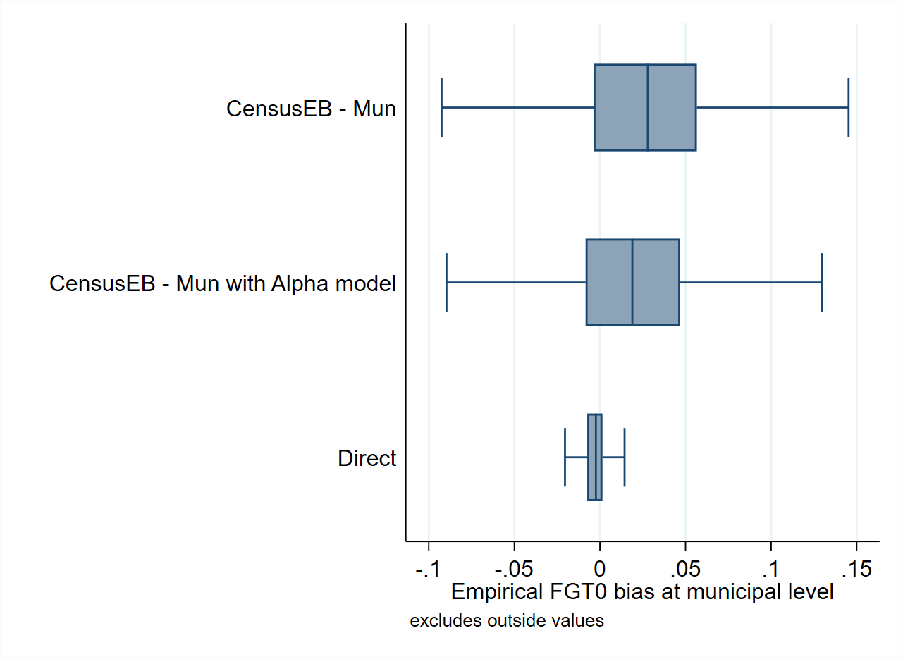
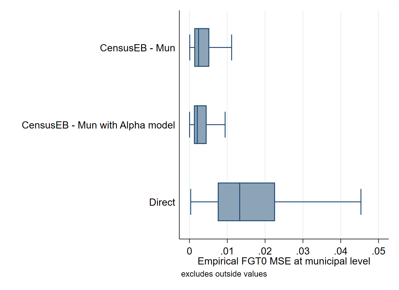
Fig. 4.8 Empirical Bias and MSE for CensusEB FGT0 estimates with and without alpha model#
Source: Based on samples of populations generated as described in Corral et al. [2021] section 4. The alpha model as specified by ELL (Elbers et al. [2002]) can be applied using the sae Package in Stata. Under the Mexican data used by Corral et al. [2021] the alpha model appears to yield positive results in terms of bias and MSE. This should be interpreted with caution as it may not be the case in other scenarios.
In practice, the implementation of the alpha model may limit modeling options for practitioners since, though available in the PovMap software, it is not included in many of the newer software packages for SAE. For example, heteroskadasticity is also considered by Molina and Rao [2010], as well as Marhuenda et al. [2017]. However, they do not specify the alpha model, and no software package implementation of their methods allows users to specify heteroskedasticity. The Stata sae package allows users to model heteroskedasticity for SAE, but only does so when using specific model fitting procedures such as the Henderson method III extension proposed by Van der Weide [2014] or the traditional ELL fitting method.27 When choosing to apply the alpha model, the Stata sae package has an option that automatically constructs the dependent variable. This dependent variable may be used to facilitate the selection of a suitable model for heteroskedasticity. A removal process of non-significant covariates may also be implemented for the alpha model, as shown in the script of Section 4.5.1.
4.2.4. Producing Small Area Estimates#
Once the model selection stage is completed, the next step is to obtain estimates for small areas. Model selection and simulation stages may be separated in different scripts to avoid re-running unnecessary processes in case of errors in only one of the stages.28 Model selection (see Stata script in Section 4.5.1) is discussed in greater detail in Chapter 6: Model Diagnostics where attention is given to the different steps involved.
The Monte Carlo simulation process can be seen in the Stata script of Section 4.5.2 and follows the model selection stage. The production of small area estimates requires first importing the census data. In Stata, it is imported into a Mata (Stata’s matrix programming language) data file, which will allow users to work with larger data sets than what is usually possible.29 The user must specify the vectors she wishes to import, including household expansion factors (typically household size) within the census data. The census data should have variable names equal to those in the survey. It is recommended to import only the necessary variables from the census to avoid creating larger data files than needed for the process.
The SAE process can be broken up into two steps. The first step entails producing the point estimates through Monte Carlo simulation. This step is relatively fast, and the recommended amount of simulations is at least 100. The estimation of the MSE is considerably more time-consuming and will usually take several hours, depending on the size of the census. Thus, it is recommended to first obtain small area estimates without specifying bootstrap simulations for MSE estimation. Once users have done their checks and determined the quality of their point estimates, the MSE can be estimated. It is recommended to use at least 200 bootstrap replications to estimate MSEs.
4.3. Pros and Cons of Unit-Level Models#
This section presents a convenient list of pros and cons for each method. It also notes the needs for each of the methods. The section borrows heavily and adds to the work presented in Molina [2019].
4.3.1. ELL#
Model requirements:
Microdata from a household survey and census at the household level, with variables measured and questions asked similarly.
A set of variables related to the welfare variable of interest. These variables should have similar distributions between the two data sources.
Areas in the survey and the census should have identifiers that can be linked across each other.
Pros:
The model is based on household-level data, which gives more detailed information than area-level data, and have a considerably larger sample size.
Can provide estimates for non-sampled areas.
Estimates from any indicator that is a function of welfare can be obtained without relying on different models.
The estimates are unbiased under the model if the model is true and the model parameters are known.
It is possible to get estimates at any level of aggregation.
Offers a software-implemented model for heteroskedasticity.
Cons:
The method, as is currently implemented, may yield rather noisy (inefficient) estimates and may even be worse than direct estimates (obtained using only the area-specific information from the survey), if heterogeneity between areas is not explained adequately.
The noise of the traditional ELL estimates is large but it is also underestimated under the ELL bootstrap procedure (see Corral et al. [2021] for details).
To reduce the above noise to the largest possible extent, it is always recommendable to include all the potentially significant covariates that may affect welfare, including contextual covariates, which may be taken from data sources different from the census.
Estimates are the outcome of a model and thus, the model needs to be appropriately checked.
The traditional ELL model specifies the location effects for the clusters (PSUs), typically nested within the areas where the estimation is desired. Estimations at higher aggregation levels than those at which the location effects are specified can underestimate noise if the area-level variables included in the model fail to explain the between-area heterogeneity.
4.3.2. Empirical Best and CensusEB#
Model requirements:
Microdata from a household survey and census at the household level with variables measured and questions asked in a similar manner.
A set of variables related to the welfare variable of interest. These variables should have similar distributions between the two data sources.
Areas in the survey and the census should have identifiers that can be linked across each other.
Pros:
Based on household-level data which provide more detailed information than area-level data and have a considerably larger sample size.
Can provide estimates for non-sampled areas.
Estimates from any indicator that is a function of welfare can be obtained without relying on different models.
Unbiased under the model, if the model is true and model parameters are known.
Optimal in the sense that they minimize the MSE under the model.
Considerably less noisy than ELL when unexplained heterogeneity across areas is considerable. For non-sampled areas, ELL and EB estimators are similar.
Offers a software-implemented model for heteroskedasticity (choosing H3 CensusEB in the Stata
saepackage).
Cons:
They are the outcome of a model and thus the model needs to be properly checked.
It may be affected by deviations from the model’s assumptions. For example, deviation from normality or outliers can have detrimental effects on SAE - isolated unit-level outliers may not have much impact if the sample size is large.
Original EB estimates do not consider the sampling design and are not design-unbiased and hence may be affected by informative sampling designs (i.e., when the sample selection probabilities depend on the outcome values - Rao and Molina Rao and Molina [2015]).
In the Stata
saepackage, the REML option obtains the original EB, but H3 CensusEB incorporates the sampling weights and should not be sensibly affected by informative sampling.
The bootstrap method for MSE estimation is computationally intensive.
4.3.3. Alternative Software Packages for Unit-Level Models and Extensions#
Packages that implement the one-fold nested-error model EB approach from Molina and Rao [2010]:
Empirical best prediction that incorporates the survey weights (Pseudo EB):
The
emdipackage in R () has been extended to include the Pseudo EB method presented in Guadarrama et al. [2018].After the updates presented in Corral et al. [2021] the
saepackage in Stata (Nguyen et al. [2018]) includes the model-fitting method that incorporates the survey weights presented in Van der Weide [2014].The implemented method only obtains CensusEB estimates.
Two-fold nested-error model EB approach as presented in Marhuenda et al. [2017]:
Estimation of area means (without transformation of welfare) based on Hierarchical Bayes unit-level models:
The
hbsaepackage in R (Boonstra [2015]).
ELL approach:
4.4. Unit-Level Models – Technical Annex#
4.4.1. The Assumed Model#
The nested-error model used for small area estimation by ELL (Elbers et al. [2003]) and Molina and Rao [2010] was originally proposed by Battese, Harter, and Fuller [1988] to produce county-level corn and soybean crop area estimates for the American state of Iowa. For the estimation of poverty and welfare, the ELL and MR methods assume the transformed welfare \(y_{ch}\) for each household \(h\) in the population within each location \(c\) is linearly related to a \(1\times K\) vector of characteristics (or correlates) \(x_{ch}\) for that household, according to the nested-error model:
Here \(\eta_{c}\) and \(e_{ch}\) are respectively location and household-specific idiosyncratic errors, assumed to be independent from each other, satisfying: $\(\eta_{c}\stackrel{iid}{\sim}N\left(0,\sigma_{\eta}^{2}\right),\:e_{ch}\stackrel{iid}{\sim}N\left(0,\sigma_{e}^{2}\right),\)$
where the variances \(\sigma_{\eta}^{2}\) and \(\sigma_{e}^{2}\) are unknown. Here, \(C\) is the number of locations in which the population is divided and \(N_{c}\) is the number of households in location \(c\), for \(c=1,\ldots,C\). Finally, \(\beta\) is the \(K\times1\) vector of coefficients.
To illustrate the differences between the methods, understanding the model is essential. First, note that the random location effect is the same for all households within a given area. Second, note that the random location effect is not necessarily 0 for a given location, despite the random location effect being drawn from a normal distribution with mean 0. Consequently, for any given realization of the population, the random location effect is unlikely to be equal to 0, but its expected value is 0 across all the possible realizations. To see this, a simulation where the random location effects for 80 areas are drawn from a normal distribution \(\eta_{c}\stackrel{iid}{\sim}N\left(0,0.15^{2}\right)\), is shown in the Stata code snippet below. This is repeated across 10,000 simulated populations.
//Do file simulates random location effects for 80 areas
set more off
clear all
version 14
set maxvar 10100

//Seed for replicability
set seed 232989
//Necessary macros
local sigmaeta = 0.15     //Sigma eta
local Npop     = 10000    //number of populations
local Narea    = 80
//Create simulated data
set obs `Narea'
//Simulate random location effects for 80 areas, 10000 populations
forval z=1/`Npop'{
	gen double eta_`z' = rnormal(0,`sigmaeta')
}
//Look at values for 1 population
sum eta_1, d //very close to 0
list eta_1 if _n==23 //not 0
//The expected value of the random location effect across populations
egen double E_eta = rmean(eta_*)
sum E_eta,d
//The expected value for one area across all populations
list E_eta if _n==23 //approximating 0
Note how in the results, the value of the random location effect for a given area and population is not necessarily equal to 0. However, across all the generated populations, the mean value of the random location effect for all areas is very close to 0.
This aspect is important, because it highlights the key difference between the methodology from ELL (Elbers et al. [2003]) and the EB approach from MR (Molina and Rao [2010]). Under ELL, when simulating welfare for the census, the location effect is drawn exactly as assumed under the model, that is as, \(\eta_{c}\stackrel{iid}{\sim}N\left(0,\sigma_{\eta}^{2}\right)\). In essence, under ELL, for any given area present in the sample, the ELL estimator of the census area mean \(\bar{y}_{c}\) is obtained by averaging the actual area means \(\bar{y}_{c}^{*(m)}=\bar{X}_{c}'\beta+\eta_{c}^{*(m)}+\bar{e}_{c}^{*(m)}\), \(m=1,\ldots,M\), across \(M\) simulated populations, that is, the ELL estimator is \(\frac{1}{M}\sum_{m=1}^{M}\bar{y}_{c}^{*(m)}\), which approximates \(E\left(\bar{y}_{c}\right)\). But note that \(E[\eta_{c}]=0\) and \(E[e_{ch}]=0\). Hence, the ELL estimator reduces to the regression-synthetic estimator, \(\bar{X}_{c}'\beta\) (MR, Molina and Rao [2010]). On the other hand, under MR (Molina and Rao [2010]), conditioning on the survey sample ensures that the estimator includes the random location effect, since \(E[\bar{y}_{c}|\eta_{c}]=\bar{X}_{c}'\beta+\eta_{c}\). suggests that the inclusion of contextual variables somewhat attenuates the issue. Nevertheless, unless the contextual variables together with the household-level ones fully explain the variation in welfare across areas, there will always be gains from using EB compared to ELL. Actually, the EB approach from Molina and Rao [2010] gives approximately the best estimator in the sense that it yields the estimator with the minimum mean squared error (MSE) for target areas. Consequently, EB estimators are considerably more efficient than ELL (see Molina and Rao [2010]; Corral et al. [2021]; and Corral et al. [2021]).
A census data set of \(N=20,000\) observations is created, similar to MR (Molina and Rao [2010]), to observe how conditioning on the survey sample affects the resulting small area estimates. Under the created data, all observations are uniformly spread among \(C=80\) areas, labeled from 1 to 80. This means that every area consists of \(N_{c}=250\) observations. The location effects are simulated as \(\eta_{c}\stackrel{iid}{\sim}N\left(0,0.15^{2}\right)\); note that every observation within a given area will have the same simulated effect. Then, values of two right-hand side binary variables are simulated. The first one, \(x_{1}\), takes a value of 1 if a generated random uniform value between 0 and 1 is less than or equal to \(0.3+0.5\frac{c}{80}\). This means that observations in areas with a higher label are more likely to get a value of 1. The next one, \(x_{2}\), is not tied to the area’s label. This variable takes the value 1 if a simulated random uniform value between 0 and 1 is less than or equal to 0.2. The census welfare vectors \(y_{c}=(y_{c,1},\ldots,y_{c,N_{c}})^{T}\) for each area \(c=1,\ldots,C\), are then created from the model as follows: \(\ln(y_{ch})=3+0.03x_{1,ch}-0.04x_{2,ch}+\eta_{c}+e_{ch},\) where household-level errors are generated under the homoskedastic setup, as \(e_{ch}\overset{iid}N\left(0,0.5^{2}\right)\). The poverty line is fixed at \(z=12\), corresponding to roughly 60 percent of the median welfare of a generated population. The steps to creating such a population in Stata are shown below:
set more off
clear all
version 14
set seed 648743

local obsnum    = 20000  //Number of observations in our "census"
local areasize  = 250    //Number of observations by area
local outsample = 20	 //Sample size from each area (%)
local sigmaeta = 0.15     //Sigma eta
local sigmaeps = 0.5      //Sigma eps


// Create area random effects
set obs `=`obsnum'/`areasize''
gen area = _n	// label areas 1 to C
gen eta  = rnormal(0,`sigmaeta')  //Generate random location effects
expand `areasize' //leaves us with 250 observations per area
sort area //To ensure everything is ordered - this matters for replicability
//Household identifier
gen hhid = _n
//Household expansion factors - assume all 1
gen hhsize = 1
//Household specific residual
gen e = rnormal(0,`sigmaeps')
//Covariates, some are corrlated to the area's label
gen x1=runiform()<=(0.3+.5*area/`=`obsnum'/`areasize'')
gen x2=runiform()<=(0.2)
//Welfare vector
gen Y_B = 3+ .03* x1-.04* x2 + eta + e

preserve
	sort hhid
	sample 20, by(area)
	keep Y_B x1 x2 area hhid
	save "$mdata\sample.dta", replace
restore

save "$mdata\thepopulation.dta", replace
The nested-error model is then fit to the population data using restricted maximum likelihood:
mixed Y_B x1 x2 || area:, reml
Linear predictions, \(X\hat{\beta}\), can also be obtained:
predict double xb, xb
Predicted random location effects, \(\hat{\eta}_{c}\), can also be obtained:
predict double eta_pred, reffects
sum eta_pred
Stata can also produce the linear prediction, \(X\hat{\beta}\), plus the estimated location effects, \(\hat{\eta}_{c}\):
predict double xb_eta, fitted
The expected values of the linear predictor \(X\hat{\beta}\), and the linear predictor that includes the predicted location effects, \(X\hat{\beta}+\hat{\eta}_{c}\), are the same. The difference between these is that \(X\hat{\beta}+\hat{\eta}_{c}\) includes the estimated location effect, and thus, a larger share of the variance is explained, which leads to minimized estimation errors for the areas.
sum Y_B xb xb_eta
At the same time, the area-specific predictions are considerably closer to the observed values:
collapse Y_B xb xb_eta, by(area)
list Y_B xb xb_eta in 1/10
4.4.2. Monte Carlo Simulation and Bootstrap Procedures Under CensusEB#
The best predictor is defined as a conditional expectation. For indicators with a complex shape, the conditional expectation defining the best predictor may not have a closed form. Regardless of the shape, the best predictor can be approximated by Monte Carlo simulation (Molina [2019]). ELL and MR’s EB approach clearly differ in the computational procedures used to estimate the indicators of interest and their noise. On the other hand, the original implementation of EB in PovMap and the sae Stata command used a similar computational approach to ELL. Under ELL and the original EB implementation in PovMap, noise and indicator estimates are all obtained with a single computational procedure. Corral et al. [2021] show that the noise estimates of the original ELL (referred to as variance by the authors) underestimate the true MSE of the indicators, despite ELL estimates being much noisier. On the other hand, the parametric bootstrap procedure from González-Manteiga et al. [2008] seems to estimate the noise (MSE) of EB estimators correctly.
For an in-depth discussion on how ELL and EB computational procedures differ, see Corral et al. [2021]. For easy interpretation, the expositions presented here do not consider survey weights or heteroskedasticity.30
4.4.2.1. Molina and Rao’s (2010) Monte Carlo Simulation Procedure for Point Estimates#
The EB method from MR (Molina and Rao [2010]) conditions on the survey sample data and thus makes more efficient use of the survey data, which contains the only available (and hence precious) information on the actual welfare. Conditioning on the survey data requires matching households across the survey and census. Matching households was required in the original EB approach introduced in MR (Molina and Rao [2010]). However, the census and sample households can not be matched in practice, except in some countries. When linking the two data sources is not possible, this sample may be appended to the population for areas where there is a sample. This is the approach taken in the original EB implementation in the sae R package by Molina and Marhuenda [2015]. In order to obtain a Monte Carlo approximation to the EB estimates using this software, estimates are obtained as a weighted average between a simulated census poverty rate for the area and the direct estimate of poverty obtained using the area’s sample. When the sample size relative to the population size for a given area is considerable, for example, 20%, using the sample observations of welfare may yield to a considerable gain in MSE. However, as noted in Fig. 4.5 in Section 4.2.1 the gain in MSE of EB over CensusEB approximates 0 as the sample size by area shrinks. When the sample is 4% of the population per area, an already quite large sample rarely encountered in real-world scenarios, the difference between the approaches is nearly zero.
To illustrate how CensusEB estimates are implemented, a 20% sample by area of the data created in Section 4.5.1 is used as a survey to which the model Equation (4.2) is fit. To obtain point estimates under Molina and Rao [2010], the authors assume that the considered unit-level model is the one that generates the data. Thus, the estimates for \(\beta,\) \(\sigma_{\eta}^{2}\), and \(\sigma_{e}^{2}\) obtained from the fitted model are kept fixed in the Monte Carlo simulation procedure used to obtain EB point estimates.31 Additionally, the predicted random location effects, \(\hat{\eta}_{c}\), are also kept fixed as a result of conditioning on the sample observations of welfare.
The first step consists in fitting the model and obtaining the parameter estimates, \(\hat{\theta}_{0}=\left(\hat{\beta_{0}},\:\hat{\sigma}_{\eta0}^{2},\:\hat{\sigma}_{e0}^{2}\right)\) which are later used to simulate vectors of welfare for all the population of households (a census of welfare).
//MonteCarlo simulation to obtain CensusEB estimates
use "$mdata\sample.dta", clear

	//fit model on the sample
	mixed Y_B x1 x2 || area:, reml

	//Obtain the necessary parameters
		local sigma_eta2 =  (exp([lns1_1_1]_cons))^2
		local sigma_e2   =  (exp([lnsig_e]_cons))^2
With these estimates in hand, it is possible to predict the random location effects, \(\eta_{c}\), as well as the shrinkage parameter, \(\gamma_{c}=\sigma_{\eta}^{2}\left(\sigma_{\eta}^{2}+\sigma_{e}^{2}/n_{c}\right)^{-1}\) and the variance of the random location effect, \(\sigma_{\eta}^{2}(1-\gamma_{c})\). Notice that \(\gamma_{c}\) will be between 0 and 1, hence the variance of the location effect will be smaller than \(\sigma_{\eta}^{2}\), which is the variance of the location effect under ELL. These model parameter estimates will then be used as true values to simulate the welfare vectors for the whole population of households.
	//Let's calculate the linear fit
	predict xb, xb

	//Get the residual to calculate the random location effect
	gen residual = Y_B - xb

	//Number of observations by area
	gen n_area = 1 //we'll add it later

groupfunction, mean(residual) sum(n_area) by(area)
	//Gamma or adjustment factor ()
	gen double gamma  = `sigma_eta2'/(`sigma_eta2'+`sigma_e2'/n_area)
	//Produce eta
	gen double eta = gamma*residual
	//variance of random location effects
	gen double var_eta = `sigma_eta2'*(1-gamma)

	keep area eta var_eta

tempfile mylocs
save `mylocs'
The next step consists in applying the estimated parameters, \(\hat{\theta}_{0},\) to generate the population vectors of welfare. Note how the same \(\hat{\beta}_{0}\) are used to produce the linear fit in every Monte Carlo simulation. Notice that the location effects are predicted from the sample from the corresponding area; thus, it is necessary to match areas across the sample and population. The next step consists in generating 100 vectors of welfare for the population units (census of welfare). Notice that here, the natural logarithm of welfare is reversed. Additionally, welfare for each household, \(h\), is drawn from \(\ln\left(y_{ch}\right)\sim N\left(x_{ch}\hat{\beta}_{0}+\hat{\eta}_{c0},\:\hat{\sigma}_{\eta0}^{2}(1-\hat{\gamma}_{c})+\hat{\sigma}_{e0}^{2}\right)\).
```stata
//Set seed for replicability
set seed 9374

//Bring in the population
use x1 x2 area hhid using "$mdata\thepopulation.dta", clear
	//obtain linear fit - e(b) is still in memory
	predict xb, xb

	//Include eta and var_eta
	merge m:1 area using `mylocs'
		drop if _m==2
		drop _m
	//to ensure replicability
	sort hhid
```

```stata
	//generate 100 vectors of welfare in the population
	forval z=1/100{
	    //Take the exponential to obtain welfare
	    gen double Y_`z' = exp(rnormal(xb + eta, sqrt(`sigma_e2'+var_eta)))
	}

```
  Input In [1]
    merge m:1 area using `mylocs'
                                ^
SyntaxError: unterminated string literal (detected at line 11)
Finally, FGT indicators (Foster et al. [1984]) are calculated for each area from the simulated census – this is done for the 100 simulated censuses. Then, the CensusEB estimate is obtained by averaging across the 100 FGT indicators obtained for the area.
	//Indicate poverty line
	gen povline = 12
	//Obtain FGTs for each area under every simulated vector
	sp_groupfunction, poverty(Y_*) povertyline(povline) by(area)
	//Average over simulations to obtain the EB estimate
	groupfunction, mean(value) by(measure area)
	//Reshape to obtain wide data at the area level
	qui:reshape wide value, i(area) j(measure) string
//Save CensusEB
save "$mdata\CensusEBfgt.dta", replace
Note that this is quite different from the method used for ELL, as implemented in PovMap and the Stata sae package.32 The steps detailed above are aligned to those applied by the command sae sim reml to obtain CensusEB estimates and are very similar to the approach under sae sim h3.
4.4.2.2. Parametric Bootstrap#
The parametric bootstrap used to estimate the MSE of the EB estimates was introduced by González-Manteiga et al. [2008]. It is the approach used by Molina and Rao [2010] and the one used in the sae R package from Molina and Marhuenda [2015], as well as in the updated Stata sae package.33 The procedure is computationally more demanding than the bootstrap procedure used in PovMap which was inspired by the MI literature. However, the parametric bootstrap procedure from González-Manteiga et al. [2008] tracks the real MSE values.
The process consists in, first, creating a population vector of welfare (i.e. census) using \(\hat{\theta}_{0}=\left(\hat{\beta_{0}},\:\hat{\sigma}_{\eta0}^{2},\:\hat{\sigma}_{e0}^{2}\right)\). Note that \(\hat{\theta}_{0}=\left(\hat{\beta_{0}},\:\hat{\sigma}_{\eta0}^{2},\:\hat{\sigma}_{e0}^{2}\right)\) are obtained from the original sample and match those from the ones used in the previous step for computing CensusEB point estimates.
//Macros used below
global povline = 12
global bs = 1 //Bootstrap replicates


//Gonzales-Manteiga et al. (2008) Bootstrap for estimating MSE
use "$mdata\sample.dta", clear

	//fit model on the sample
	mixed Y_B x1 x2 || area:, reml

	//Obtain the necessary parameters
		local sigma_eta2 =  (exp([lns1_1_1]_cons))^2
		local sigma_e2   =  (exp([lnsig_e]_cons))^2
	//Let's calculate the linear fit
	predict xb, xb
	dis sqrt(`sigma_eta2')
	dis sqrt(`sigma_e2')

tempfile sample
save `sample'
Using \(\hat{\theta}_{0}=\left(\hat{\beta_{0}},\:\hat{\sigma}_{\eta0}^{2},\:\hat{\sigma}_{e0}^{2}\right)\) as the vector of true values, \(B\) population vectors of welfare are created following the DGP from Equation (4.2). Each area’s desired set of indicators is obtained from each population vector. These indicators are regarded as the true values in each bootstrap replicate and the benchmark to which CensusEB estimates for that generated population will be compared to. The estimate of the MSE is the mean across the \(B\) replicates of the squared differences between the bootstrap replicate’s estimate and the bootstrap replicate’s “true” value. In the code below, the steps for the first bootstrap replicate, \(b=1,\) in this parametric bootstrap procedure are shown.
//We import the population/census data to a mata file for obtaining CensusEB
//estimates for each bootstrap replicate with sae command
preserve
	sae data import, datain("$mdata\thepopulation.dta") ///
	varlist(x1 x2 hhsize) area(area) uniqid(hhid) ///
	dataout("$mdata\mypop_mata")
restore
//Set seed for replicability
set seed 9374

local bs=1
	//Now we generate the eta vector of our population
	clear
	set obs 80 //80 areas
		gen area = _n
		gen eta_1 = rnormal(0,sqrt(`sigma_eta2'))
	tempfile etas
	save `etas'

	//Bring in the entire population (i.e. census)
	use x1 x2 area hhid hhsize using "$mdata\thepopulation.dta", clear
		//obtain linear fit - e(b) is still in memory
		predict xb, xb
		//Include the etas
		merge m:1 area using `etas'
			drop _m

		//generate welfare vector, by adding linear fit and location effect
		// and adding the idiosyncratic errors
		//Take the exponential to obtain welfare
		gen double Y_1 = exp(rnormal(xb + eta_1,sqrt(`sigma_e2')))

		//From this simulated population, which follows exactly the model's
		// assumptions the true poverty rate for the population is obtained
		gen povline = $povline
		//Obtain FGTs for each area under every simulated vector
		// This yields 200 FGTs per area
		sp_groupfunction, poverty(Y_1) povertyline(povline) by(area)
		qui:reshape wide value, i(area) j(measure) string
	tempfile true
	save `true'
Note
The part above was ommited in guidelines*
*===============================================================================
//The second stage consists in "extracting the sample" and obtaining estimates
// via MonteCarlo simulation. For each bootstrap replicate...this is b=1
*===============================================================================
	use x1 x2 xb hhid area using `sample', clear
		//Include the etas
		//note that these are the same used in the population
		merge m:1 area using `etas'
			drop _m
		sort hhid
		//Generate the welfare vector, in exactly the same manner as in the
		//population
		gen lny = rnormal(xb + eta_1,sqrt(`sigma_e2'))

	local seedstage  `c(rngstate)'

	// Now with the new welfare vector we can obtain CensusEB estimates
	//for the bootstrap replicate using sae
	sae sim reml lny x1 x2,  area(area)  mcrep(50) bsrep(0) lny ///
	seed(`seedstage') pwcensus(hhsize) indicators(FGT0 FGT1 FGT2) ///
	aggids(0) uniq(hhid) plines($povline) matin("$mdata\mypop_mata")

	//MSE is calculated as squared difference between the true and CensusEB.
	//Bring in the true poverty for this bootstrap replicate
	rename Unit area
	merge 1:1 area using `true'
		drop _m
	//Get squared difference, after B bootstrap replicates the sum of these
	// squared differences is our MSE estimate
	forval a = 0/2{
	    gen sq_diff_fgt`a' = ((avg_fgt`a' - valuefgt`a')^2)/$bs
	}
/*
	keep area sq_diff_fgt*

	if (`bs'==1){
		rename  sq_diff_fgt* MSE_fgt*
		tempfile mse
		save `mse'
	}
	else{
	    merge 1:1 area using `mse'
			drop _m
		forval a = 0/2{
			replace MSE_fgt`a' = MSE_fgt`a' + sq_diff_fgt`a'
		}
		tempfile mse
		save `mse'
	}

use `mse', clear
Note
The second part above was ommited in guidelines*
4.5. Appendix#
4.5.1. Model Selection Do-File#
This do-file provides an example of the steps that may be followed to select a model for SAE, according to the discussion from Section 4.2. The steps for model checking follow those illustrated by UCLA’s Statistical Consulting Group ().
clear all
set more off

/*===============================================================================
Do-file prepared for SAE Guidelines
- Real world data application
- authors Paul Corral & Minh Nguyen
*==============================================================================*/

global main     "C:\Users\\`c(username)'\OneDrive\SAE Guidelines 2021\"
global section  "$main\3_Unit_level\"
global mdata    "$section\1_data\"
global survey "$mdata\survey_public.dta"
global census "$mdata\census_public.dta"

//global with candidate variables.
global myvar rural  lnhhsize age_hh male_hh  piped_water no_piped_water ///
no_sewage sewage_pub sewage_priv electricity telephone cellphone internet ///
computer washmachine fridge television share_under15 share_elderly ///
share_adult max_tertiary max_secondary HID_* mun_* state_*


version 15
set seed 648743

*===============================================================================
// End of preamble
*===============================================================================
//load in survey data
use "$survey", clear
	//Remove small incomes affecting model
	drop if e_y<1
	//Log shift transformation to approximate normality
	lnskew0 double bcy = exp(lny)
	//removes skeweness from distribution
	sum lny, d
	sum bcy, d

	//Data has already been cleaned and prepared. Data preparation and the creation
	// of eligible covariates is of extreme importance.
	// In this instance, we skip these comparison steps because the sample is
	// literally a subsample of the census.
	codebook HID //10 digits, every single one
	codebook HID_mun //7 digits every single one

	//We rename HID_mun
	rename HID_mun MUN
	//Drop automobile, it is missing
	drop *automobile* //all these are missing

	//Check to see if lassoregress is installed, if not install
	cap which lassoregress
	if (_rc) ssc install elasticregress

	//Model selection - with Lasso
	gen lnhhsize = ln(hhsize)
	lassoregress bcy  $myvar [aw=Whh], lambda1se epsilon(1e-10) numfolds(10)
	local hhvars = e(varlist_nonzero)
	global postlasso  `hhvars'

	//Try Henderson III GLS
	sae model h3 bcy $postlasso [aw=Whh], area(MUN)

	//Rename HID_mun
	rename MUN HID_mun

	//Loop designed to remove non-significant covariates sequentially
	forval z= 0.5(-0.05)0.05{
		qui:sae model h3 bcy `hhvars' [aw=Whh], area(HID_mun)
		mata: bb=st_matrix("e(b_gls)")
		mata: se=sqrt(diagonal(st_matrix("e(V_gls)")))
		mata: zvals = bb':/se
		mata: st_matrix("min",min(abs(zvals)))
		local zv = (-min[1,1])
		if (2*normal(`zv')<`z') exit

		foreach x of varlist `hhvars'{
			local hhvars1
			qui: sae model h3 bcy `hhvars' [aw=Whh], area(HID_mun)
			qui: test `x'
			if (r(p)>`z'){
				local hhvars1
				foreach yy of local hhvars{
					if ("`yy'"=="`x'") dis ""
					else local hhvars1 `hhvars1' `yy'
				}
			}
			else local hhvars1 `hhvars'
			local hhvars `hhvars1'
		}
	}

	global postsign `hhvars'

	//Henderson III GLS - model post removal of non-significant
	sae model h3 bcy $postsign [aw=Whh], area(HID_mun)

	//Check for multicollinearity, and remove highly collinear (VIF>3)
	reg bcy $postsign [aw=Whh],r
	cap drop touse 	//remove vector if it is present to avoid error in next step
	gen touse = e(sample) 		//Indicates the observations used
	vif 						//Variance inflation factor
	local hhvars $postsign
	//Remove covariates with VIF greater than 3
	mata: ds = _f_stepvif("`hhvars'","Whh",3,"touse")
	global postvif `vifvar'

	//VIF check
	reg bcy $postvif [aw=Whh], r
	vif

	//Henderson III GLS - model post removal of non-significant
	sae model h3 bcy $postvif [aw=Whh], area(HID_mun)

*===============================================================================
// 2.5 Model checks
*===============================================================================

	reg bcy $postvif
	predict cdist, cooksd
	predict rstud, rstudent

	reg bcy $postvif [aw=Whh]
	local KK = e(df_m)
	predict lev, leverage
	predict eps, resid
	predict bc_yhat, xb

	//Let's take a look at our residuals
	//Notice there is a downward sloping line,which seems to be the smallest eps for that xb
	scatter eps bc_yhat
	//so we can see what the figure looks like
	sleep 15000
	// so there's a bunch of small incomes that may be affecting our model!
	scatter eps bc_yhat if exp(lny)>1

/* https://stats.idre.ucla.edu/stata/dae/robust-regression/
Residual:  The difference between the predicted value (based on the regression ///
equation) and the actual, observed value.

Outlier:  In linear regression, an outlier is an observation with large ///
residual.  In other words, it is an observation whose dependent-variable ///
value is unusual given its value on the predictor variables.  An outlier may ///
indicate a sample peculiarity or may indicate a data entry error or ///
other problem.

Leverage:  An observation with an extreme value on a predictor variable is a ///
point with high leverage.  Leverage is a measure of how far an independent ///
variable deviates from its mean.  High leverage points can have a great ///
amount of effect on the estimate of regression coefficients.

Influence:  An observation is said to be influential if removing the ///
substantially changes the estimate of the regression coefficients.  ///
Influence can be thought of as the product of leverage and outlierness.

Cook’s distance (or Cook’s D): A measure that combines the information of ///
leverage and residual of the observation
*/

/* Rules of thumb:
Cooks -> >4/N, also according to "Regression Diagnostics: An Expository ///
Treatment of Outliers and Influential Cases, values over 1...

Abs(rstu) -> >2 We should pay attention to studentized residuals that exceed ///
+2 or -2, and get even more concerned about residuals that exceed +2.5 or ///
-2.5 and even yet more concerned about residuals that exceed +3 or -3.  ///

leverage ->	>(2k+2)/n
*/
	hist cdist, name(diag_cooksd, replace)
	hist lev, name(diag_leverage, replace)
	hist rstud, name(diag_rstudent, replace)
	twoway scatter cdist lev, name(diag_cooksd_lev, replace)

	lvr2plot, name(lvr2)
	rvfplot, name(rvf)

	sum cdist, d
	local max = r(max)
	local p99 = r(p99)

	reg lny $postvif [aw=Whh]
	local myN=e(N)
	local myK=e(rank)

	//We have influential data points...
	reg lny $postvif if cdist<4/`myN' [aw=Whh]
	reg lny $postvif if cdist<`max'   [aw=Whh]
	reg lny $postvif if cdist<`p99'   [aw=Whh]
	gen nogo = abs(rstud)>2 & cdist>4/`myN' & lev>(2*`myK'+2)/`myN'


*===============================================================================
// Selecting the Alpha model
*===============================================================================
	//Rename HID_mun
	cap rename HID_mun MUN
	//Henderson III GLS - add alfa model
	sae model h3 bcy $postvif if nogo==0 [aw=Whh], area(MUN) ///
	alfatest(residual) zvar(hhsize)

	des residual_alfa //The dependent variable for the alfa model

	// Macro holding all eligible vars
	unab allvars : $myvar
	//Macro with current variables
	local nogo $postvif

	//We want to only use variables not used
	foreach x of local allvars{
		local in = 0
		foreach y of local nogo{
			if ("`x'"=="`y'")	local in=1
		}
		if (`in'==0) local A `A' `x'
	}

	global A `A' //macro holding eligible variables for alpha model

	lassoregress residual_alfa `A' if nogo==0 [aw=Whh]

	local alfa = e(varlist_nonzero)
	global alfa `alfa'

	reg residual_alfa $alfa if nogo==0 [aw=Whh],r
	gen tousealfa = e(sample)

	//Remove vif vars
	mata: ds = _f_stepvif("$alfa","Whh",5,"tousealfa")

	global alfa `vifvar'

	//Alfa vars before removal of non-significant vars
	global beforealfa `alfa'

	local hhvars $alfa

	forval z= 0.9(-0.1)0.1{
		foreach x of varlist `hhvars'{
			local hhvars1
			qui: reg residual_alfa `hhvars' [aw=Whh], r
			qui: test `x'
			if (r(p)>`z'){
				local hhvars1
				foreach yy of local hhvars{
					if ("`yy'"=="`x'") dis ""
					else local hhvars1 `hhvars1' `yy'
				}
			}
			else local hhvars1 `hhvars'
			local hhvars `hhvars1'

		}
	}
	global alfavars `hhvars'

	//Henderson III Model with alpha model
	sae model h3 bcy $postvif if nogo==0 [aw=Whh], area(MUN) zvar($alfavars)

*===============================================================================
// GLS model, one final removal of non-significant variables
*===============================================================================
	//Loop designed to remove non-significant covariates sequentially
	local hhvars $postvif
	forval z= 0.5(-0.05)0.05{
		qui:sae model h3 bcy `hhvars' if nogo==0 [aw=Whh], area(MUN) ///
		zvar($alfavars)
		mata: bb=st_matrix("e(b_gls)")
		mata: se=sqrt(diagonal(st_matrix("e(V_gls)")))
		mata: zvals = bb':/se
		mata: st_matrix("min",min(abs(zvals)))
		local zv = (-min[1,1])
		if (2*normal(`zv')<`z') exit

		foreach x of varlist `hhvars'{
			local hhvars1
			qui:sae model h3 bcy `hhvars' if nogo==0 [aw=Whh], area(MUN) ///
			zvar($alfavars)
			qui: test `x'
			if (r(p)>`z'){
				local hhvars1
				foreach yy of local hhvars{
					if ("`yy'"=="`x'") dis ""
					else local hhvars1 `hhvars1' `yy'
				}
			}
			else local hhvars1 `hhvars'
			local hhvars `hhvars1'
		}
	}

	global postalfa `hhvars'

*===============================================================================
// SAVE the data with the pertinent covariates and other info
*===============================================================================
sae model h3 bcy $postalfa if nogo==0 [aw=Whh], area(MUN) zvar($alfavars)

char _dta[rhs]   $postalfa
char _dta[alpha] $alfavars
char _dta[sel]   nogo

save "$mdata\mysvy.dta", replace
4.5.2. SAE Simulation Stage#
This do-file provides an example of the steps commonly followed to produce the final CensusEB small area estimates. It follows the discussion from Section 4.2.4.
clear all
set more off

/*===============================================================================
Do-file prepared for SAE Guidelines
- Real world data application
- authors Paul Corral & Minh Nguyen
*==============================================================================*/

global main     "C:\Users\\`c(username)'\OneDrive\SAE Guidelines 2021\"
global section  "$main\3_Unit_level\"
global mdata    "$section\1_data\"
global survey "$mdata\survey_public.dta"
global census "$mdata\census_public.dta"

version 15
local seed 648743

*===============================================================================
// End of preamble
*===============================================================================
use "$mdata\mysvy.dta", clear
	char list

	global hhmodel : char _dta[rhs]
	global alpha   : char _dta[alpha]
	global sel     : char _dta[sel]

//Add lnhhsize
use "$census"
gen lnhhsize = ln(hhsize)

tempfile census1
save `census1'

// Create data ready for SAE - optimized dataset
sae data import, datain(`census1') varlist($hhmodel $alpha hhsize) ///
area(HID_mun) uniqid(hhid) dataout("$mdata\census_mata")

*===============================================================================
// Simulation -> Obtain point estimates
*===============================================================================
use "$mdata\mysvy.dta", clear
	drop if e_y<1
	drop if $sel==1
	rename MUN HID_mun
sae sim h3 e_y $hhmodel, area(HID_mun) zvar($alpha) mcrep(100) bsrep(0) ///
lnskew matin("$mdata\census_mata") seed(`seed') pwcensus(hhsize) ///
indicators(fgt0 fgt1 fgt2) aggids(0 4) uniqid(hhid) plines(715)

*===============================================================================
// Simulation -> Obtain MSE estimates
*===============================================================================

use "$mdata\mysvy.dta", clear
	drop if e_y<1
	drop if $sel==1
	rename MUN HID_mun
sae sim h3 e_y $hhmodel, area(HID_mun) zvar($alpha) mcrep(100) bsrep(0) ///
lnskew matin("$mdata\census_mata") seed(`seed') pwcensus(hhsize) ///
indicators(fgt0 fgt1 fgt2) aggids(0 4) uniqid(hhid) plines(715)

save "$mdata\mySAE.dta", replace
4.6. References#
- BDL+06
Abhijit V Banerjee, Angus Deaton, Nora Lustig, Kenneth Rogoff, and Edward Hsu. An evaluation of world bank research, 1998-2005. Available at SSRN 2950327, 2006.
- BHF88(1,2)
George E. Battese, Rachel M. Harter, and Wayne A. Fuller. An error-components model for prediction of county crop areas using survey and satellite data. Journal of the American Statistical Association, 83(401):28–36, 1988. URL: http://www.jstor.org/stable/2288915.
- Boo15
Harm Jan Boonstra. Package 'hbsae'. R Package Version, 2015.
- BC64
GEP Box and DR Cox. An analysis of transformations. Journal of the Royal Statistical Society, Series B, 26:211–252, 1964.
- CHMM21(1,2,3,4,5,6,7,8,9,10,11,12,13,14,15)
Paul Corral, Kristen Himelein, Kevin McGee, and Isabel Molina. A map of the poor or a poor map? Mathematics, 2021. URL: https://www.mdpi.com/2227-7390/9/21/2780, doi:10.3390/math9212780.
- CMN21(1,2,3,4,5,6,7,8,9,10,11,12,13,14,15,16,17,18,19,20,21)
Paul Corral, Isabel Molina, and Minh Cong Nguyen. Pull your small area estimates up by the bootstraps. Journal of Statistical Computation and Simulation, 91(16):3304–3357, 2021. URL: https://www.tandfonline.com/doi/abs/10.1080/00949655.2021.1926460, doi:10.1080/00949655.2021.1926460.
- EFL+07
Chris Elbers, Tomoki Fujii, Peter Lanjouw, Berk Ozler, Wesley Yin, and others. Poverty alleviation through geographic targeting: how much does disaggregation help? Journal of Development Economics, 83(1):198–213, 2007.
- ELL03(1,2,3,4,5)
Chris Elbers, Jean O Lanjouw, and Peter Lanjouw. Micro–level estimation of poverty and inequality. Econometrica, 71(1):355–364, 2003.
- ELL02(1,2,3,4,5,6,7)
Chris Elbers, Jean Olson Lanjouw, and Peter Lanjouw. Micro-level estimation of welfare. World Bank Policy Research Working Paper, 2002.
- FGT84
James Foster, Joel Greer, and Erik Thorbecke. A class of decomposable poverty measures. Econometrica: Journal of the Econometric Society, 52:761–766, 1984.
- GonzalezMLombardiaM+08(1,2,3,4)
Wenceslao González-Manteiga, Maria J Lombardía, Isabel Molina, Domingo Morales, and Laureano Santamaría. Bootstrap mean squared error of a small-area EBLUP. Journal of Statistical Computation and Simulation, 78(5):443–462, 2008.
- GMR18
María Guadarrama, Isabel Molina, and JNK Rao. Small area estimation of general parameters under complex sampling designs. Computational Statistics & Data Analysis, 121:20–40, 2018.
- Har76
Andrew C Harvey. Estimating regression models with multiplicative heteroscedasticity. Econometrica: Journal of the Econometric Society, 44:461–465, 1976. URL: https://www.jstor.org/stable/1913974?casa_token=rLCctNWylroAAAAA:3-S22Hv84lze8TUU-3nyFgDGZsrxkAoCZHwUVKO99Qynn_zXmr8-3kmdqFxdLxRBJT8KiE-xYwfoI5-gzFA9RF3N-KHS3g7na1Soi8WbYp_QBcPfjU7m&seq=1.
- Hen53(1,2,3)
Charles R Henderson. Estimation of variance and covariance components. Biometrics, 9(2):226–252, 1953.
- MMMR17(1,2,3,4,5,6)
Yolanda Marhuenda, Isabel Molina, Domingo Morales, and JNK Rao. Poverty mapping in small areas under a twofold nested error regression model. Journal of the Royal Statistical Society: Series A (Statistics in Society), 180(4):1111–1136, 2017. doi:10.1111/rssa.12306.
- MNS+20
Takaaki Masaki, David Newhouse, Ani Rudra Silwal, Adane Bedada, and Ryan Engstrom. Small area estimation of non-monetary poverty with geospatial data. World Bank Policy Research Working Paper, 2020.
- Mol19(1,2,3)
Isabel Molina. Desagregación De Datos En Encuestas De Hogares: Metodologías De Estimación En áreas Pequeñas. CEPAL, 2019. URL: https://repositorio.cepal.org/handle/11362/44214.
- MM15(1,2,3,4,5,6,7,8)
Isabel Molina and Yolanda Marhuenda. Sae: an R package for small area estimation. The R Journal, 7(1):81–98, 2015.
- MR10(1,2,3,4,5,6,7,8,9,10,11,12,13,14,15,16,17)
Isabel Molina and JNK Rao. Small area estimation of poverty indicators. Canadian Journal of Statistics, 38(3):369–385, 2010.
- NCAZ18(1,2,3,4,5,6,7,8,9)
Minh Cong Nguyen, Paul Corral, João Pedro Azevedo, and Qinghua Zhao. Sae: a stata package for unit level small area estimation. World Bank Policy Research Working Paper, 2018.
- PC19
Ryan A Peterson and Joseph E Cavanaugh. Ordered quantile normalization: a semiparametric transformation built for the cross-validation era. Journal of Applied Statistics, 47(13-15):2312–2327, 2019. URL: https://www.tandfonline.com/action/showCitFormats?doi=10.1080/02664763.2019.1630372, doi:10.1080/02664763.2019.1630372.
- RM15(1,2,3)
JNK Rao and Isabel Molina. Small Area Estimation. John Wiley & Sons, 2nd edition, 2015.
- RPPST20
Natalia Rojas-Perilla, Sören Pannier, Timo Schmid, and Nikos Tzavidis. Data-driven transformations in small area estimation. Journal of the Royal Statistical Society: Series A (Statistics in Society), 183(1):121–148, 2020.
- TZL+18(1,2,3)
Nikos Tzavidis, Li-Chun Zhang, Angela Luna, Timo Schmid, and Natalia Rojas-Perilla. From start to finish: a framework for the production of small area official statistics. Journal of the Royal Statistical Society: Series A (Statistics in Society), 181(4):927–979, 2018.
- VdW14(1,2,3,4,5)
Roy Van der Weide. GLS estimation and empirical bayes prediction for linear mixed models with heteroskedasticity and sampling weights: A background study for the POVMAP project. World Bank Policy Research Working Paper, 2014. URL: https://papers.ssrn.com/sol3/papers.cfm?abstract_id=2495175.
- Zha06(1,2,3,4)
Qinghua Zhao. User Manual for Povmap. 2006. URL: http://siteresources. worldbank. org/INTPGI/Resources/342674-1092157888460/Zhao_ ManualPovMap. pdf.
4.7. Notes#
- 1
This section draws from the background papers for these guidelines. See Corral et al. [2021] and Corral et al. [2021].
- 2
A factor that likely contributed to the expansion of these methods is the availability of software, which can be easily used to apply these approaches;
PovMap(Zhao [2006]) for ELL and R’ssaepackage (Molina and Marhuenda [2015]). While other methods exist, for the purposes of this section, attention is given to the methods noted.- 3
It is highly recommended that novice practitioners start by reading Section 4.1.1.
- 4
Stata’s double-precision only goes up to 16 digits.
- 5
Additional information is provided in the technical annex Section 4.4.
- 6
Interested readers can refer to Stata’s documentation to learn more about mixed models.
- 7
To see the help file in Stata type:
help sae_ebpfor the one-fold nested-error model.- 8
CensusEB estimates are similar to EB estimates, but do not include survey observations when calculating small area estimates. See Molina [2019] or Corral et al. [2021] for more details.
- 9
To see help file in Stata type:
help sae_ebp2for the two-fold nested-error model.- 10
Methods that do not consider the survey sampling weights may in turn include covariates that capture the sampling/response mechanism, trying to correctly model their relationship to the target variable.
- 11
To see help file in Stata type:
help sae_mc_bsfor the one-fold nested-error model fit with Henderson’s method III heteroskedasticity and survey weights (see Van der Weide [2014]).- 12
Readers may refer to Elbers et al. [2002] or Nguyen et al. [2018] for a full exposition of the alpha model for heteroskedasticity.
- 13
The adaptation was made in light of criticism regarding the fitting method described in ELL (Elbers et al. [2002]). See Nguyen et al. [2018] for more details.
- 14
Ensuring the use of same area identifiers is still recommended for the inclusion of area-level variables.
- 15
To see help file in Stata type:
help sae_ellfor the one-fold nested-error model fit with heteroskedasticity and survey weights (see Van der Weide [2014]).- 16
Corral et al. [2021] discuss the differences between the methods used for noise estimation and how the methods fare when applied to simulated data.
- 17
Section 4.4 gives a more detailed explanation on the differences.
- 18
Empirical MSE are obtained from multiple samples. Under model-based simulations, the sample is kept fixed, and across populations the only difference is in the errors. Under design-based simulations, multiple samples are taken from a single (fixed) population.
- 19
In areas with no information (areas not sampled), EB and ELL estimates are similar.
- 20
The implementation of the ELL method in PovMap allowed practitioners to draw errors from the empirical distribution, which in principle may benefit the method when normality does not hold. Nevertheless, when comparing CensusEB method (assuming normal errors) and ELL method (drawing errors from the empirical distribution) in a model-based simulation experiment, where the model errors used to generate the populations were drawn from a Student’s t-distribution, CensusEB outperformed ELL by a considerable margin (see Corral et al. [2021]).
- 21
In cases where, even after transformation, the deviation is apparent only in isolated observations or isolated areas, models based on mixtures of normal distributions may be used. To estimate poverty and inequality indicators, a mixture may be specified as done by . extend the EB procedure to a multivariate mixture model that incorporates heterogeneity in the regression coefficients apart from the variance components. The proposed model was used to estimate FGT0 and FGT1 by gender in West Bank and Gaza.
- 22
R packages
sae(Molina and Marhuenda [2015]) andemdi() also incorporate transformations.- 23
Refer to the help files for
bcskew0andlnskew0to learn more about the transformation.- 24
An alternative approach to modeling heteroskedasticity is to consider a random coefficient model similar to the one studied in and applied to the estimation of mean income. However, the method has not been implemented in any software.
- 25
The example shows lower bias and a smaller MSE for a particular data set and could not translate equally to other data sets.
- 26
Heteroskedasticity may be checked by plotting residuals against predicted values.
- 27
In terms of alternatives, the R package
mcmcsae() can also model heteroskedasticity in terms of covariates.- 28
It is advisable to split the processes across multiple do files, because model selection, as well as simulating welfare in the cesus and obtaining small area estimates for all areas is not computationally negligible.
- 29
Note Stata cannot open this data file as a regular dta file.
- 30
For the full exposition, see Corral, Molina, and Nguyen [2021].
- 31
Note that this is considerably different from the approach that was implemented in
PovMapCorral et al. [2021].- 32
See Corral et al. [2021] for more details.
- 33
See Corral et al. [2021] for more details.