Poverty Mapping in Off-Census Years
Contents
5. Poverty Mapping in Off-Census Years#
Considerable attention has been given to produce reliable poverty maps in off-census years. An updated poverty map is increasingly becoming an essential resource to improve the targeting of many social protection programs around the world, which was underscored by the rapid onset and widespread impact of the COVID-19 crisis. Even in the best-case scenarios, poverty maps that rely on unit-level small area estimation techniques combining a census and survey can only be obtained once a decade. In off-census years, the typical small area approach applied has been an area-level model, such as a Fay-Herriot or a sub-area-level model, such as the one proposed by Torabi and Rao [2014]). Nevertheless, since the perceived gains in precision from area-level models are less than stellar, methods that combine unit- and area-level models have been proposed (see Nguyen [2012]; Lange et al. [2018]; Masaki et al. [2020]). These models are here called unit-context models and, although appealing, seem to yield considerably biased estimates.
Beyond the small area estimation literature, the machine learning literature has made several contributions to poverty mapping. Recent research in this area include Chi et al. [2021] and Jean et al. [2016]. The authors of these two papers created highly disaggregated poverty maps by modeling the direct estimates of an asset index at a very low geographical level (e.g. villages or enumeration areas) using satellite-derived covariates. The authors of those papers rely on machine learning approaches, such as gradient boosting and ridge regression, to obtain estimates for small areas. These models provide point estimates of poverty at a low geographical level, although they do not necessarily provide an adequate estimate of the method’s noise. The methods are attractive since they present the possibility of producing a poverty map even when a contemporaneous or reliable census does not exist.
5.1. Unit-Context Models#
Unit-context models attempt to model the population’s welfare distribution using only area-level covariates. More specifically, unit-context models combine unit and area-level information to model the transformed household-level welfare (unit) using only area-level covariates (context). Since unit-context models do not require census microdata, they have been proposed as an alternative approach for the case when the available census microdata is too outdated to be considered for use under the conventional model-based methods that include unit-level covariates.1
Previous applications of unit-context models for small area estimation were proposed by , who studied the number of trips home students have taken, and by , who looked at batting averages and toxoplasmosis cases. In these applications, the method appears to work well, although in both studies, the model with aggregate covariates is used to produce estimates of the area means of the dependent variable in the model (no transformation is considered). In the context of poverty, the target poverty indicators are typically complex nonlinear functions of the dependent variables in the model. Hence, properly replicating the full welfare distribution is essential as noted in Fig. 4.1. At the area level, this is complicated since household characteristics are not used in the model. Thus very little, if any, of the variation in welfare across households in the area is explained. If simple area means of the welfare variable of interest are the target, then, due to the assumptions embedded into the nested-error models used in Chapter 4: Unit-level Models for Small Area Estimation, a transformation (such as log or log-shift) of the welfare variable is used as the dependent variable in the model. Consequently, the area means of the untransformed welfare variable are desired, which are then means of exponentials of the dependent variable. As is illustrated in the next section, when estimating indicators that are nonlinear functions of the dependent variables in the model, unit-context models will likely produce small area estimators of poverty with substantial bias.
Nguyen [2012] first considered unit-context models for poverty estimation in an application for Vietnam. In this application, the dependent variable was the household-level logarithm of per capita expenditure from the Vietnam Household Living Standard Survey from 2006, whereas all covariates are commune-level means obtained from a dated (1999) census. Nguyen [2012] obtains ELL estimates of poverty for small areas under that model and compares the performance with typical ELL poverty estimates obtained using unit-level covariates from the Vietnam Household Living Standard Survey from 2006 and the 2006 Rural Agriculture and Fishery Census. The author finds that provinces and districts hovering around the middle of the distribution suffered considerable re-rankings across methods. However, those at the top and the bottom were relatively stable.
A similar approach to the one from Nguyen [2012] was presented by Lange et al. [2018] as an alternative in cases when census and survey data are not from similar periods. However, the same inefficiency issues noted in Chapter 4: Unit-level Models for Small Area Estimation regarding ELL estimates would likely persist when considering a model using only area-level covariates. Improvements to the approach were seemingly made by Masaki et al. [2020] by taking measures to address some of the shortcomings of a standard ELL approach and to obtain EB estimators from Molina and Rao [2010]. The authors conduct a design-based validation study using census data for Sri Lanka and Tanzania for a wealth index constructed by principal component analysis and suggest that the use of EB improves precision over ELL when implementing unit-context models.
Although the unit-context approach is attractive in that it does not require a contemporaneous census and can readily accommodate variables extracted from the emerging fields related to geospatial analysis, there are serious concerns about bias in unit-context estimators, as noted in Corral et al. [2021] as well as the concerns raised in the following section. The MSE from unit-context models is also likely to be incorrectly estimated since the required parametric bootstrap procedure assumes the underlying model using only area-level characteristics to be correct. In other words, the unit-context model’s assumptions require household-level welfare to not depend on household-specific characteristics, which is unlikely to be the case. Incorrect MSE estimates risk presenting a map with considerable bias as being overly precise. Therefore, based on the currently available evidence, area-level models, like Fay-Herriot (Chapter 3: Area-level Models for Small Area Estimation), are generally preferred over unit-context models (see the following section for more details).
In cases where neither area- nor unit-level models are advised due to data limitations, no clear consensus has emerged on the best path forward or if one even exists. In evaluating alternatives, practitioners should choose methods which rely on assumptions that are realistic to the circumstances in which the model will be employed, which are approximately unbiased (or its bias does not exceed a certain limit), and for which an accurate method exists to measure the small area estimators’ MSE. In cases where the MSE cannot be adequately estimated, then at least it should be known in which (realistic) scenarios the approach has limited bias. If these conditions cannot be reasonably met, it is preferable to not produce a map than to produce one with potentially biased estimates, or one in which precision is overestimated, or most worrisome, both. In the next section, the limitations of unit-context models are discussed.
5.1.1. Limitations of Unit-Context Models#
Based on results from a validation study using model- and design-based simulations, Corral et al. [2021] conclude unit-context models, like those presented in Masaki et al. [2020], Lange et al. [2018] and Nguyen [2012] are not recommended except under exceptional cases due to the high likelihood of bias in estimates.2
Nguyen [2012] application of a unit-context model to estimate poverty in small areas in Vietnam already hints toward potential problems of the unit-context approach. The author compares the results from unit-context models to those obtained via a standard unit-level method, ELL, and finds considerable changes in rankings. Nguyen [2012] finds that differences in rankings are largest for locations around the middle of the distribution.
Despite the use of EB, the unit-context application by Masaki et al. [2020], also provides hints of potential methodological problems with the approach. A ratio procedure was used to benchmark the values to ensure alignment between direct estimates at the level of representativeness and the estimates obtained by the approach. The need to benchmark indicates considerable discrepancies between the sum of estimated totals at the lower level and the estimated total at the higher level. The need to benchmark also suggests that the model’s assumptions are not satisfied.

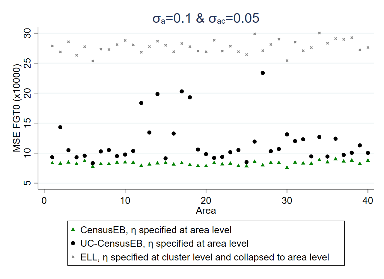
Fig. 5.1 Empirical Bias and MSE for CensusEB based on a unit-level model and CensusEB based on a unit-context model (UC-CensusEB) and ELL FGT0 estimates from model based simulations#
Source: Corral et al. [2021]. The figure is obtained from simulations based on 10,000 populations and samples as specified in Corral et al. [2021]. The simulations illustrate that unit context (UC) model may yield FGT0 estimates that are upward biased and with MSEs that could be several orders of magnitude above those of CensusEB estimates, based on the analogous unit-level model, and for some areas may be almost as inefficient as ELL.
Unit-context models appear to yield upward biased FGT0 estimates in model-based simulations, as presented in Fig. 5.1 (most areas show bias above 0). Since unit-context models are special cases of the models used in ELL and EB procedures (see Section 4.4.1), but without household-level characteristics, the between-household variation of welfare is not adequately explained by the model. Corral et al. [2021] suggest that part of the observed bias comes from this misspecification, with effects similar to omitted variable bias (OVB) (see the appendix in Corral et al. [2021]). Despite the bias, the empirical MSE of unit-context models seems to outperform that of ELL estimates (Fig. 5.1).
Like traditional unit-level models, unit-context models also assume normally distributed errors and departures from normality may also produce bias (which might offset or compound the previous bias). This is why in Section 4.2.2, a considerable emphasis is placed on data transformation, all with the aim of approximating the normality assumption. Because of the poor model fit and potential deviations from normality, unit-context models also display considerable bias when estimating mean welfare (see Fig. 5.2).
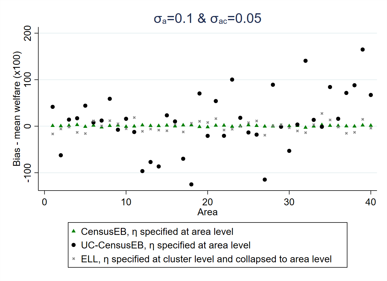
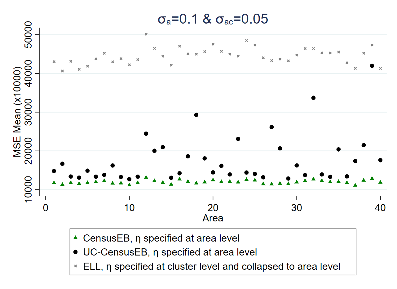
Fig. 5.2 Empirical Bias and MSE for CensusEB based on a unit-level model and CensusEB based on a unit-context model (UC-CensusEB) and ELL mean welfare estimates from model based simulations#
Source: Corral et al. [2021]. The figure is obtained from simulations based on 10,000 populations and samples as specified in Corral et al. [2021]. The simulations illustrate that unit-context models may yield mean welfare estimates that are considerably biased and with MSEs that could be several orders of magnitude above those of CensusEB estimates based on the analogous unit-level model and for some areas may be as inefficient as ELL.
In the simulation results displayed in Fig. 5.2, the dependent variable is the natural log of welfare. Nevertheless, what practitioners are often interested in is welfare, and hence need to reverse the log transformation. Since \(\exp\left[E\left(\ln y\right)\right]\neq E\left(y\right)\). The log linear nested-error model (\(\ln y_{ch}=x_{ch}\beta+\eta_{c}+e_{ch}\)) implies that \(y_{ch}=\exp\left(x_{ch}\beta\right)\exp\left(\eta_{c}\right)\exp\left(e_{ch}\right)\), then \(E\left(y_{ch}|x_{ch}\right)=\exp\left(x_{ch}\beta\right)E\left[\exp\left(\eta_{c}\right)\right]E\left[\exp\left(e_{ch}\right)\right]\). Since it is assumed that \(\eta_{c}\sim N\left(0,\sigma_{\eta}^{2}\right)\) and \(e_{ch}\sim N\left(0,\sigma_{e}^{2}\right)\), then \(E\left[\exp\left(\eta_{c}\right)\right]=\exp\left(0.5\sigma_{\eta}^{2}\right)\) and \(E\left[\exp\left(e_{ch}\right)\right]=\exp\left(0.5\sigma_{e}^{2}\right)\). Because unit-context models do not include household-level covariates, the resulting estimate of \(\sigma_{e}^{2}\) is likely much greater than the true \(\sigma_{e}^{2}\). This implies that unit-context models may yield an upward biased prediction of mean household welfare for the area despite the use of EB methods since unbiasedness is assured for the area means of \(\ln y\) but not for those of \(y\) following back transformation.
To illustrate this last point, a simulation where the modeling and estimates are obtained using the same source is conducted (see Appendix Section 5.5.1.2). This is done to remove the potential source of bias noted in the Appendix of Corral et al. [2021]. The empirical bias of the estimators in each of the 40 areas in the census data set are represented in box-plots. First, note that, when estimating the area means of the dependent variable (similar to when no transformation is taken), the biases of the CensusEB estimators based on the unit-context model are not that large (Fig. 5.3, left). However, suppose one estimates the means of the untransformed welfare variable (exponential of the model’s dependent variable). In that case, the incorrect estimate of \(\sigma_{\eta}^{2}+\sigma_{e}^{2}\) plays a considerable role, and thus the estimates of mean welfare based on unit-context models are upward biased despite the use of EB methods (Fig. 5.3, right). As shown in Fig. 5.3 (right), the average bias of CensusEB estimators based on unit-context models is considerable. For some areas, the bias may be over 800 times the bias of the CensusEB estimators based on the analogous unit-level models.
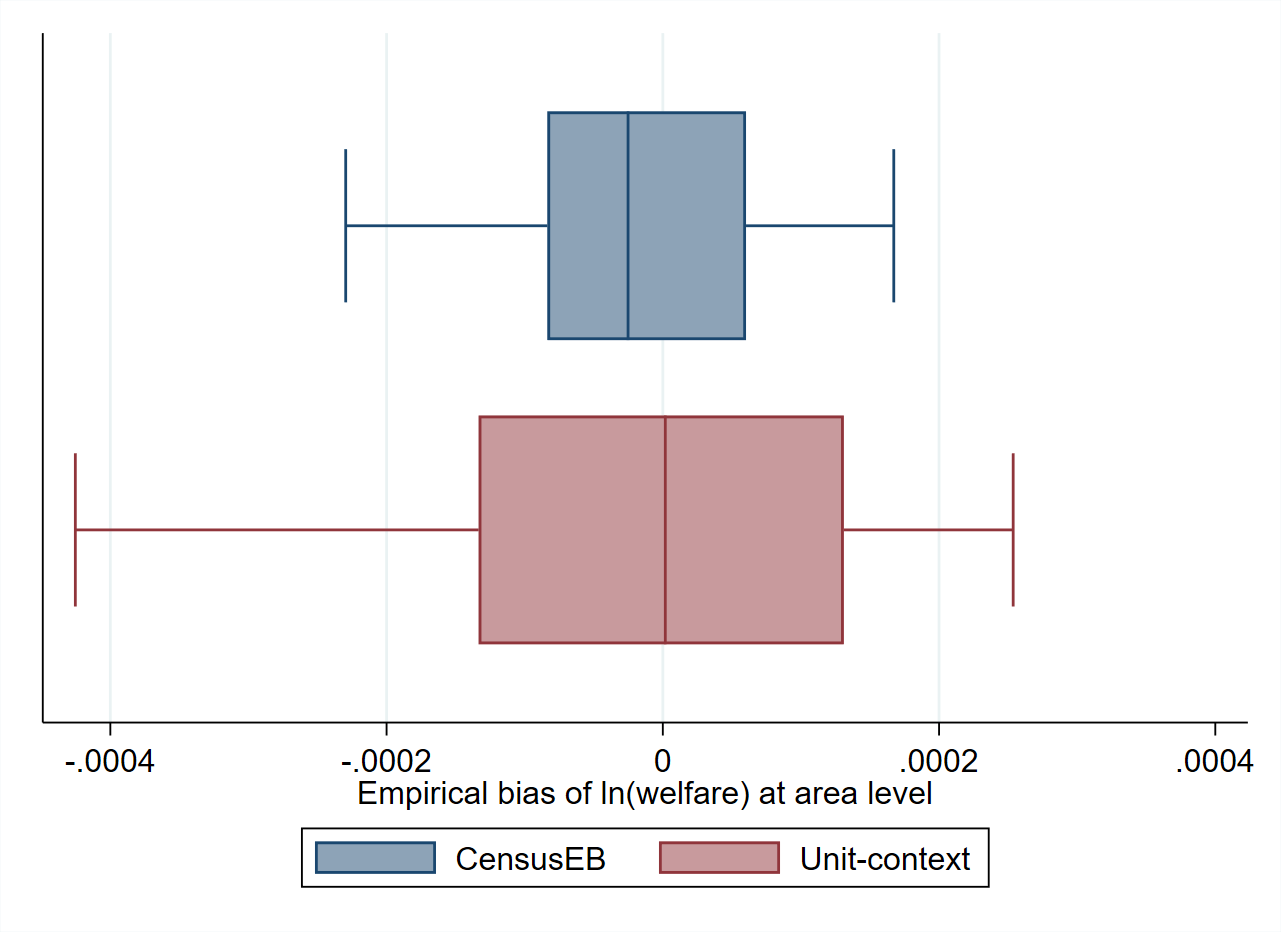
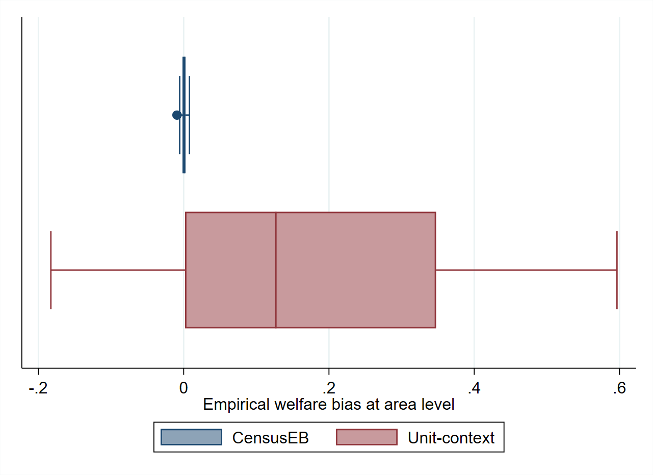
Fig. 5.3 Empirical Bias of CensusEB prediction of the area means of \(ln(y_ais)\), left, and \(y_ais\), right, obtained from a unit-level model and from a unit-context model#
Note: Simulation based on 5,000 populations generated as described in Section 5.5.1. The model is fit to the whole population and then welfare is simulated for the same population to yield 5,000 EB predictors for each area. Box-plots represent the empirical bias for the 40 areas in the census data. Do-file to replicate simulation can be seen in Section 5.5.1.1.
The source of bias discussed, i.e. due to biased estimators of the variance components under unit-context models, is in addition to the bias due to the difference between the sample and census means of the covariates noted in Corral et al. [2021]. The latter source of bias is not relevant here as it is related to sampling, and in this case, the entire census is taken as the sample. The bias due to variance components will affect the estimation of mean welfare and headcount poverty. Consequently, estimates of headcount poverty under unit-context models will be biased also because of poor model fit. As shown in Fig. 5.4, the estimates from the unit-context models are upward biased for all areas, which occurs because the full distribution of the population is not accurately replicated under unit-context models.
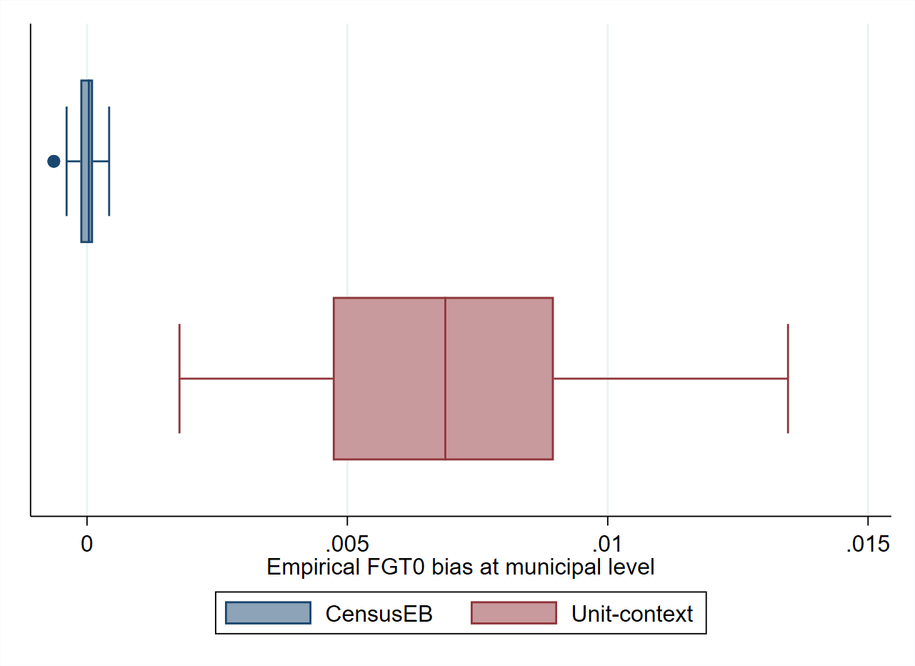
Fig. 5.4 Empirical Bias of CensusEB predictors of FGT0 under unit-level model and under a unit-context model#
Note: Simulation based on 5,000 populations generated as shown in section. The model is fit on the entire population and then welfare is simulated on the same population to yield 5,000 EB predictors for each area. Box-plot represents the empirical bias for the 40 areas in the census data. Do-file to replicate simulation can be seen in Section 5.5.1.1.
A potentially significant difference between the results presented in Fig. 5.3 and Fig. 5.4, and the applications of Masaki et al. [2020] and Lange et al. [2018] is the considerably lower \(R^{2}\) of the unit-context models presented here. To address the low \(R^{2}\), the simulation experiment is repeated using a slightly modified data generating process leading to an increase of the model’s \(R^{2}\) (Technical Annex Section 5.5.1). This modification leads to an \(R^{2}\) of the unit-context model between 0.15 and 0.20, while for the unit-level model the \(R^{2}\) exceeds 0.60. This adjustment in the data generating process reduces the bias in the estimators of mean welfare based on the unit-context model (Fig. 5.5), but the direction of the bias is different from that of the original simulation (Fig. 5.2). This change of direction of the bias also occurs when estimating poverty rates, and the direction of the bias seems to change with the poverty threshold. Estimators based on unit-context models are upward biased for poverty rates under a threshold of 13. If this threshold is increased to 28, the unit-context estimators of the poverty rate become downward biased for every area (Fig. 5.6). These results illustrate a crucial shortcoming of unit-context models: in a given application, a practitioner cannot know which will be the direction and the magnitude of the bias. Unit-context models seldom reproduce the true distribution accurately, and it is difficult to know in which cases they work properly.
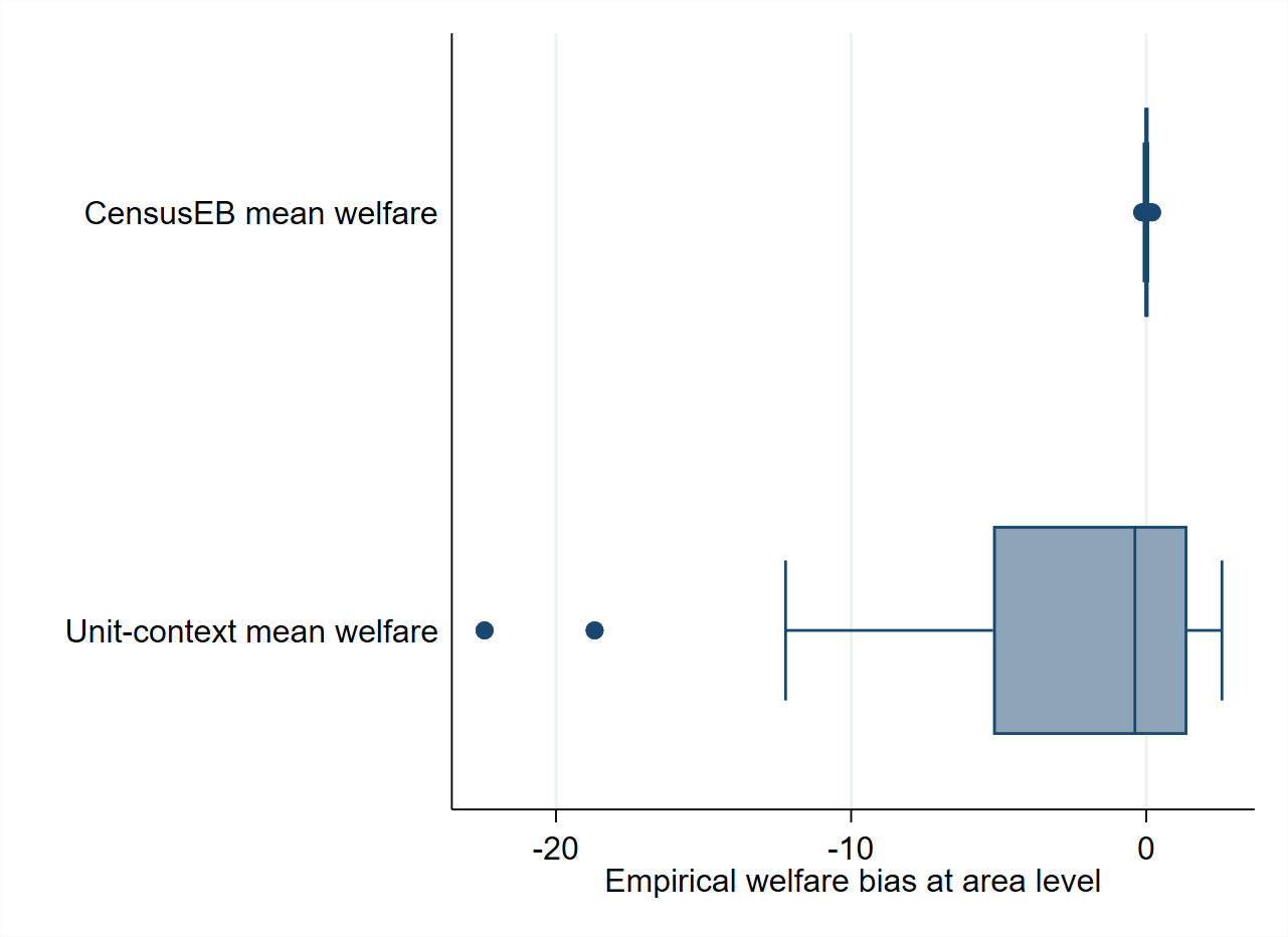
Fig. 5.5 Empirical Bias of CensusEB predictors under unit-level model and under a unit-context model#
Note: Simulation based on 5,000 populations generated as shown in Section 5.5.1. The model is fit on the entire population and then welfare is simulated on the same population to yield 5,000 EB predictors for each area. Box-plot represents the empirical bias for the 40 areas in the census data. Do-file to replicate simulation can be seen in Section 5.5.1.2.
Building upon the previous simulation, a final simulation is conducted to observe how unit-context models perform under 99 different poverty thresholds. The thresholds correspond to the 99 percentiles of the first population generated in the simulation (detailed in Appendix Section 5.5.2). In contrast to the previous simulations, a sample from the population is taken here. This is done to compare unit-context estimators to estimators based on an FH model (Chapter 3: Area-level Models for Small Area Estimation).
As expected, the unit-level CensusEB estimator yields the smallest bias across all areas and poverty lines (Fig. 5.7). The shape of the bias for unit-context models suggests that it may perform well for some poverty lines, while it will perform poorly for other poverty lines. This agrees with what is noted in Fig. 5.6, where the method could work for a given poverty line but show substantial bias at a different poverty threshold. Moreover, for many areas and poverty lines, unit-context models seem to perform worse than FH models, not just with respect to bias but also in terms of empirical MSE (Fig. 5.8).
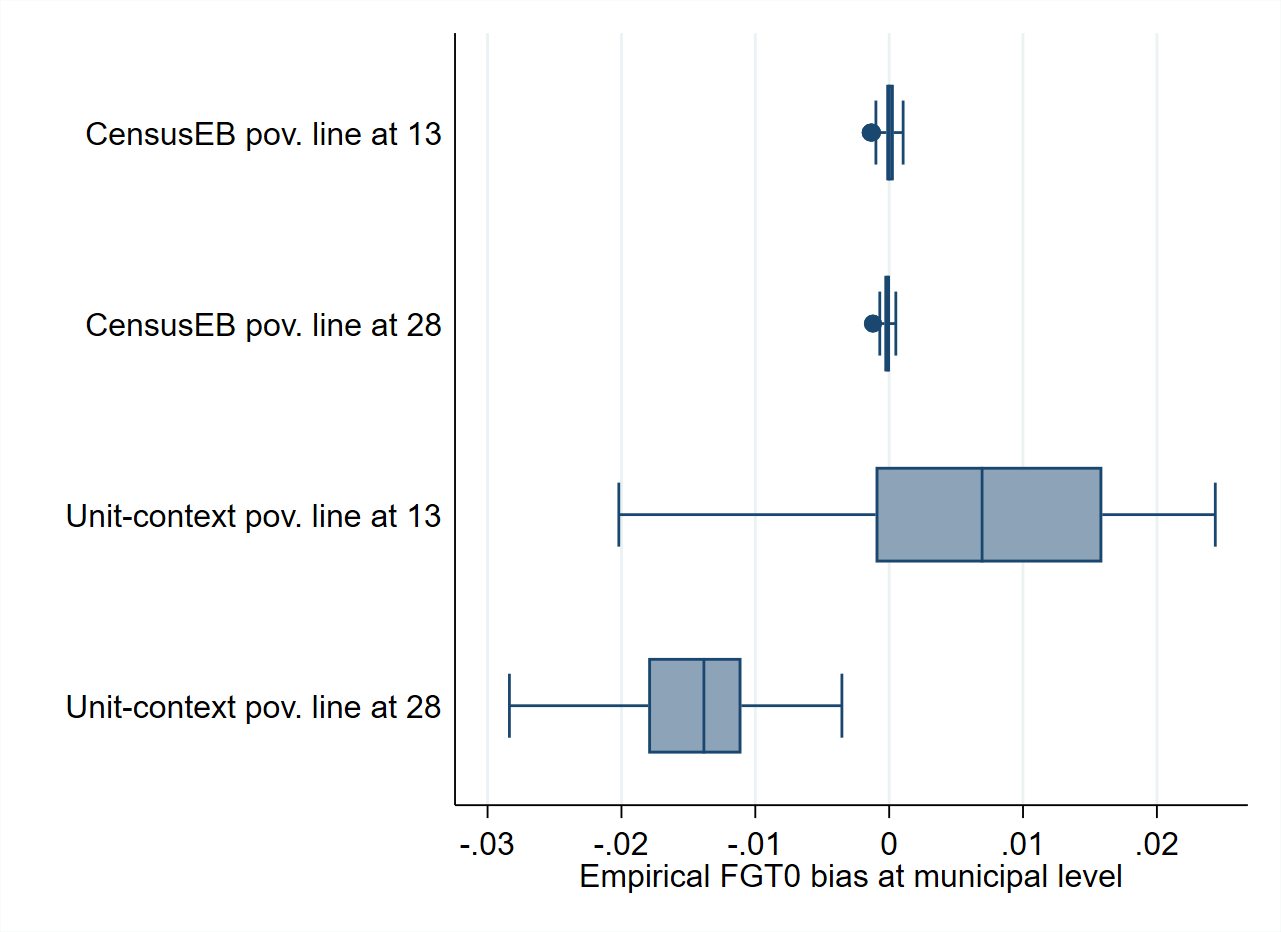
Fig. 5.6 Empirical Bias of CensusEB predictors of FGT0 under unit-level model and under a unit-context model#
Note: Simulation based on 5,000 populations generated as shown in Section 5.5.1. The model is fit on the entire population and then welfare is simulated on the same population to yield 5,000 EB predictors for each area. Box-plot represents the empirical bias for the 40 areas in the census data. Do-file to replicate simulation can be seen in Section 5.5.1.2.
The average absolute empirical bias can be used to rank the different methods. Across all 99 poverty lines, unit-context models have the highest average absolute empirical bias (Fig. 5.9).3 Additionally, the average empirical MSE (across the 100 areas) for each poverty line is surprisingly close between Fay-Herriot and unit-context models. However, neither dominates the other (Fig. 5.10), supporting the conclusion that unit-context models should be used with caution and only when unit-level and area-level options are not feasible. If unit-context models are used, all caveats should be made clear to the users of the resulting estimates.
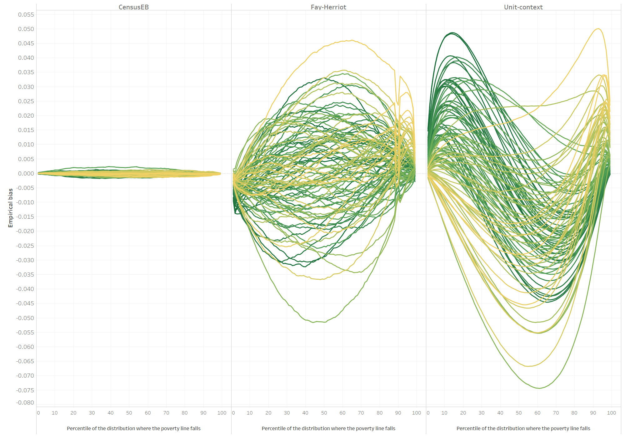
Fig. 5.7 Empirical bias of different methods for each area and poverty line#
Note: Simulation based on 1,000 populations generated as described in this section. Each line corresponds to one of the 100 areas. The x-axis represents the percentile on which the poverty line falls on, and the y-axis is the empirical bias. In instances where direct estimates have a variance of 0 and hence FH estimates cannot be obtained, the direct estimate is used as the FH estimate for that area. The do-file to replicate these results can be found in Section 5.5.2.1.
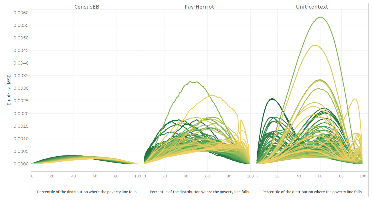
Fig. 5.8 Empirical MSE of different methods for each area and poverty line#
Note: Simulation based on 1,000 populations generated as described in this section. Each line corresponds to one of the 100 areas. The x-axis represents the percentile on which the poverty line falls on, and the y-axis is the empirical MSE. In instances where direct estimates have a variance of 0 and hence FH estimates cannot be obtained, the direct estimate is used as the FH estimate for that area. The do-file to replicate these results can be found in Section 5.5.2.1.
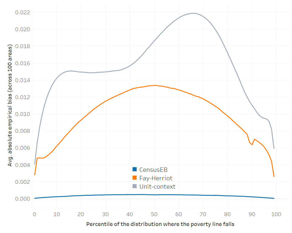
Fig. 5.9 Average absolute empirical bias of different methods for each poverty line#
Note: Simulation based on 1,000 populations generated as described in this section. Each line corresponds to the average across 100 areas of the absolute empirical bias for each method. The x-axis represents the percentile on which the poverty line falls on, and the y-axis is the average absolute empirical bias. In instances where direct estimates have a variance of 0 and hence FH estimates cannot be obtained, the direct estimate is used as the FH estimate for that area. The do-file to replicate these results can be found in Section 5.5.2.1.
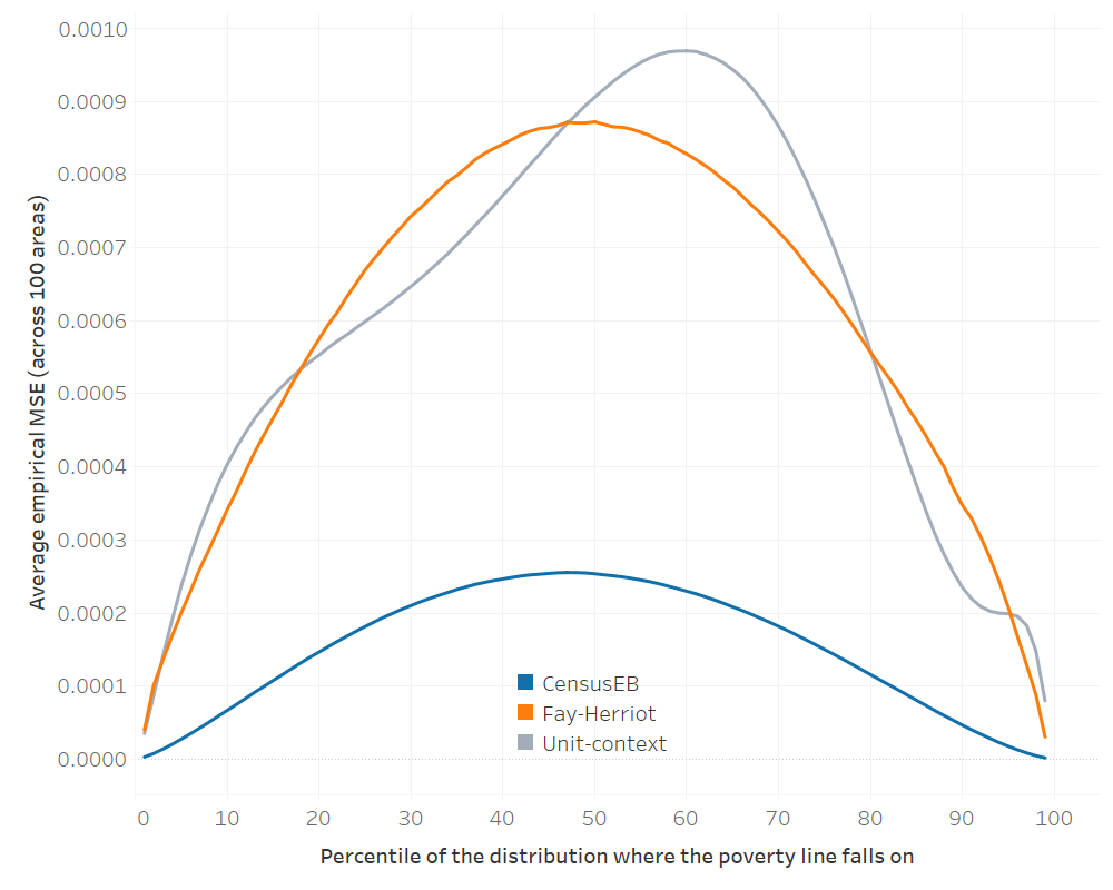
Fig. 5.10 Average empirical MSE of different methods for each poverty line#
Note: Simulation based on 1,000 populations generated as described in this section. Each line corresponds to the average across 100 areas of the mean squared error for each method. The x-axis represents the percentile on which the poverty line falls on, and the y-axis is the average MSE. In instances where direct estimates have a variance of 0 and hence FH estimates cannot be obtained, the direct estimate is used as the FH estimate for that area. The do-file to replicate these results can be found in Section 5.5.2.1.
In addition to bias, there are concerns with an overstatement of precision from a unit-context model. If welfare depends on household-level characteristics (which is expected) the MSE estimates of CensusEB estimators based on unit-context models, obtained using the parametric bootstrap procedure of González-Manteiga et al. [2008], would not be appropriate as it may underestimate the method’s true MSE by a considerable amount. The parametric bootstrap procedure under the unit-context model is done considering that the unit-context model is the true data generating process and thus generates bootstrap populations from that model. However, this assumption is shown to not hold in the simulation experiment, leading to inaccurate MSE estimates (Fig. 5.11). Consequently, under unit-context models, one can produce biased poverty estimates but may be presented as being very precise.
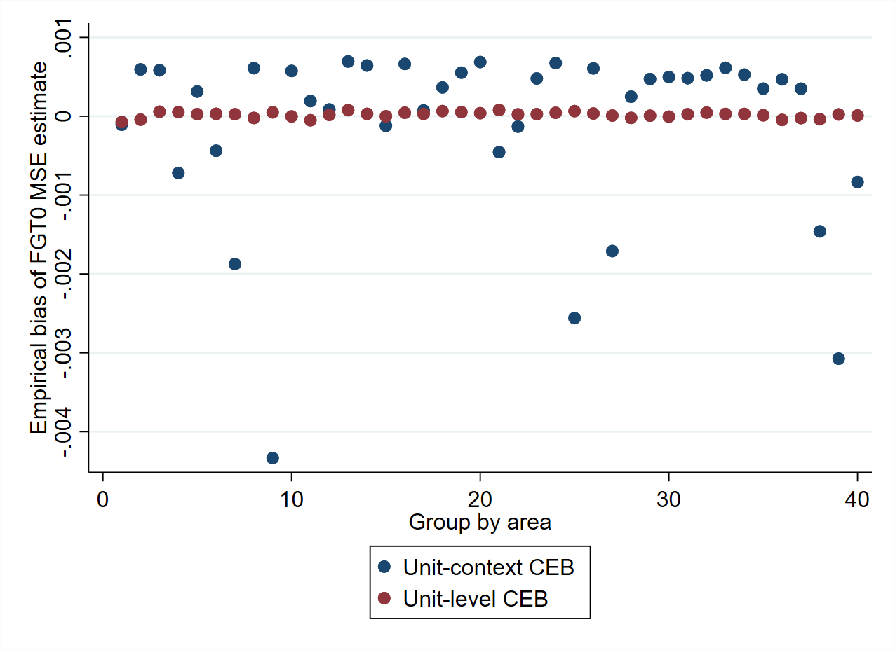
Fig. 5.11 Bias of parametric MSE estimate by method#
Note: Simulation based on 1,000 populations generated as described in this section. Under each population, MSE estimates are obtained using the parametric bootstrap procedure of González-Manteiga et al. [2008]. The empirical MSE is compared to the estimated MSE to obtain the bias of the MSE estimates of each method.
Summarizing concerns with unit-context models, given the limitations of unit-context models, even under an ideal scenario where the model is fit to the whole set of population data and EB estimates are obtained also using the population data, unit-context models should be considered only if unit-level and area-level options have been exhausted. While it is possible that in real world applications, there may be bias from multiple sources which offset each other out for a given poverty threshold, there is no way for an analyst to determine if biases are canceling or compounding each other as the direction of the bias is not known a priori. A likely overstatement of precision further complicates this unknown bias. This situation recalls an original concern levied against ELL by Banerjee et al. [2006] where the authors state: “What we are most concerned about is the possibility that the Bank is making very attractive poverty maps, whose precision is not known, but which come with statements of precision that we suspect may be seriously misleading. In the worst case scenario, a map that may be worthless is presented as one that is extremely precise” (Banerjee et al. [2006], pg 61).
5.2. Gradient Boosting for Poverty Mapping#
With the advent of increased computing power, machine learning approaches have gained popularity in the literature as well as in policy circles. For example, poverty estimates for small areas derived from a gradient boosting application by Chi et al. [2021] guided the expansion of social protection in Nigeria; specifically, the estimates were used as an input to the Rapid Response Register for the COVID-19 Cash Transfer Project.4
Gradient boosting methods rely on, first, creating a linear fit (usually a constant term) to the data at hand and then fitting a new model onto the residuals. In contrast to ensemble techniques, the multiple fits are not averaged. Instead, the predicted residuals (scaled by a learning rate) are added to the previous step’s prediction, successively taking small steps using the same or different covariates at each step toward the final prediction. This process repeats until the requested number of predictions are completed, or there is no longer a gain in prediction.5 A complete exposition of the approach is beyond the scope of the Guidelines, and interested readers can refer to or Chen and Guestrin [2016] for a more nuanced description of the approach.
A validation approach similar to the one done by Corral et al. [2021] is implemented to test how well gradient boosting works in a poverty mapping context. Specifically, 500 samples taken from the census created from the Mexican Intercensal Survey are used to conduct a design-based simulation experiment to validate the method.6 The Mexican Intercensal Survey is uniquely suited for this validation since it includes a measure of income at the household level and is representative at the municipal level and localities with 50,000 or more inhabitants. The survey was modified to obtain a census dataset of 3.9 million households and 1,865 municipalities Corral et al. [2021]. Using a sampling approach similar to the one used for Living Standards Measurement Study (LSMS) surveys, 500 samples are drawn from the resulting census.
In each of the 500 samples, a model is fit. The model’s dependent variable is the direct estimator of the headcount poverty rate at the PSU level (or municipality), and PSU aggregates (or municipality) from the census data are used as covariates. The models are fit using the XGBoost algorithm available in Python and R.7 Introduced by Chen and Guestrin [2016], XGBoost is a scalable machine learning system for tree boosting and is available as an open-source software library. To make the comparison fair, for each of the 500 samples, a model is selected using lasso regression as detailed in Section 6.2 and fit for the considered small area estimation methods. This is different from the approach usually taken under design-based validation, where one model is considered the true model and is used across all samples. The results for the XGBoost and the SAE methods are illustrated in Fig. 5.12. The results illustrate that in the case of the Mexican data, XGBoost yields unbiased estimates of poverty. Moreover, the empirical MSE compares favorably with that of CensusEB methods, which are more computational and data-intensive. Additionally, in this Mexican scenario, the gradient boosted estimates are superior to those from the unit-context method discussed in the previous section (labeled U-C CensusEB).
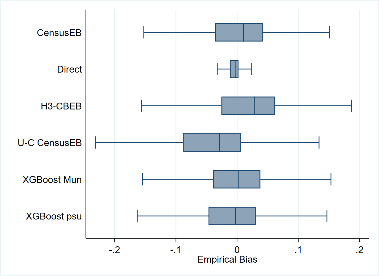
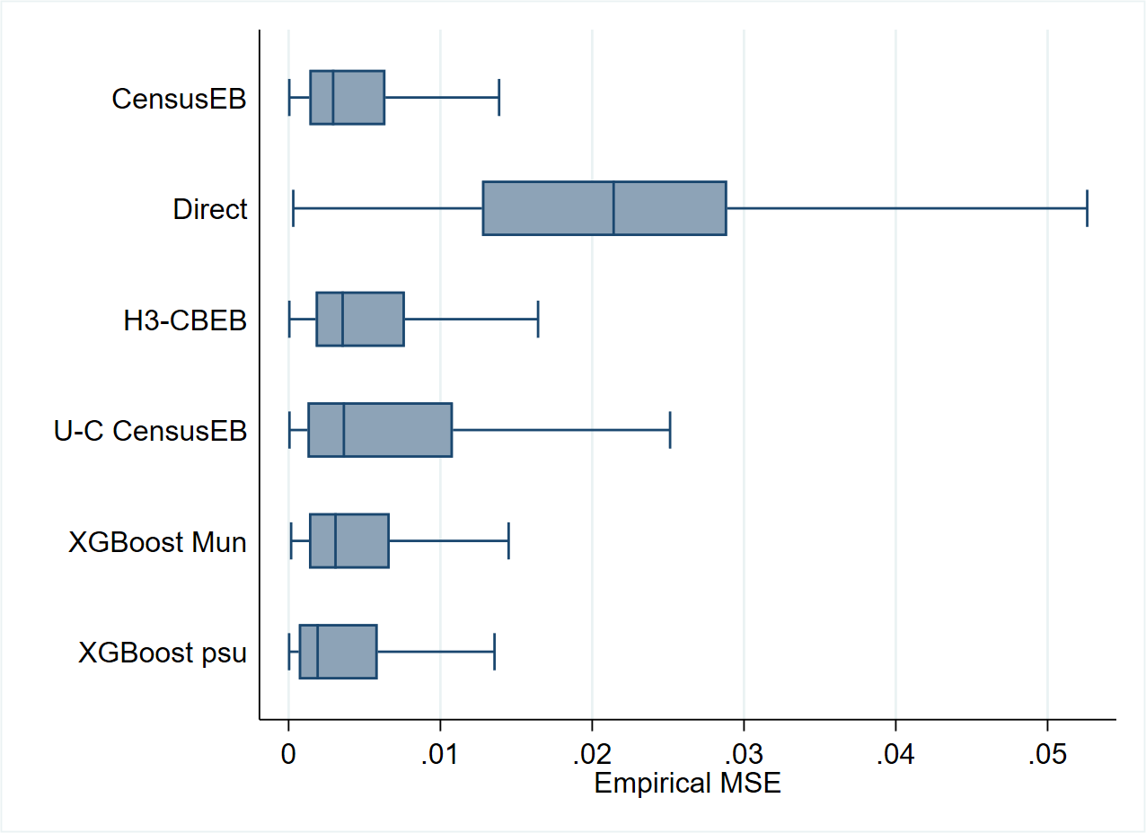
Fig. 5.12 Empirical bias and MSE of FGT0 for different methods#
Source: Data from Corral et al. [2021]. The simulations are based on 500 samples taken from the Mexican Intercensal survey, which is treated as a census of 3.9 million households. Under each sample, predictors for each of the methods are obtained and then compared to the true values obtained from the Mexican Intercensal survey. The figure illustrates that in the Mexican Intercensal case, XGBoost yields FGT0 estimates that are very close in performance, in terms of bias and MSE, to those from CensusEB estimators based on a unit-level model. H3-CBEB is the clustered bootstrap EB which is discussed in detail in Corral et al. [2021], the method was the EB approach implemented in PovMap and the original sae Stata package.
Despite the gradient boosting method’s performance, it also carries some caveats. First, though the method performs well with the Mexican data, there is uncertainty as to the degree to which these results can be extrapolated to other contexts.8 Second, there are currently no implemented software options for estimating the method’s MSE.9 Finally, despite XGBoost being based on open-source software, it is still somewhat of a black box and not easily interpretable. Therefore, further research is required to properly assess how well the method works, though early results are encouraging.
5.3. Pros and Cons of Methods for Poverty Mapping in Off-Census Years#
This section presents a convenient list of pros and cons for each method discussed in this chapter. It also notes the needs for each of the methods. The section is borrows from Molina [2019].
5.3.1. Unit-Context Models#
Model requirements:
Microdata from a household survey (only the model’s dependent variable) and administrative, satellite-derived data, or any other area or sub-level data.
Masaki et al. [2020] recommend using data that is at least one level below the level at which results are to be presented, although the more disaggregated, the better.
The population size/count at the area level is needed, at least the number of dwellings in the area.
Areas and sub-areas in the survey and the census should have identifiers that can be linked.
Pros:
Based on household-level welfare from a survey and area-level data from any point in time. It may be used in off census years, avoiding the use of outdated census data.
Unlike Fay-Herriot area-level models (Fay III and Herriot [1979]), it can be applied for areas with an estimated sampling variance equal to 0.
May provide estimates for non-sampled areas.
Cons:
The welfare model is presumably incorrectly specified unless household-level welfare is dependent only on area-level characteristics. Hence, estimates are expected to be biased, and the direction and magnitude of the bias are unknown a priori.
The bootstrap method for MSE estimation is computationally intensive.
The parametric bootstrap approach from González-Manteiga et al. [2008] under the unit-context model is likely to yield an inaccurate measure of MSE. In many instances, the MSE may be considerably underestimated.
5.3.2. Gradient Boosting#
Model requirements:
Direct estimates of indicators of interest for the areas considered, \(\hat{\tau}_{d}^{DIR}\) (from the survey).
Aggregate data at the area level of all necessary covariates for the model for every area considered, \(\mathbf{x}_{d}\), \(d=1,\ldots,D\).
Areas in the survey and the census should have identifiers that can be linked across each other.
Pros:
Based on direct estimates from a survey and area-level data from any point in time. It may be used in off census years, avoiding the use of outdated census data.
Unlike Fay-Herriot area-level models (Fay III and Herriot [1979]), it can be applied for areas with an estimated sampling variance equal to 0.
The method’s dependent variable and the target indicators are the same. In a design-based simulation using the Mexican Intercensal Survey the method yields estimates of comparable quality to CensusEB and with better performance than unit-context models.
May provide estimates for non-sampled areas.
Cons:
The method requires validation exercises in more scenarios beyond the one conducted in this chapter. There is no guarantee that the method will work as well with covariates with considerably lower predictive power than the ones from the example provided in Section 5.2.
The method currently lacks an approach for obtaining noise estimates (MSE). Consequently, it is difficult to assess the precision of the final estimates.
5.4. Unit-Context Models – Technical Annex#
5.4.1. Producing Estimators Based on Unit-Context Models#
The production of estimators based on unit-context models is similar to those using regular unit-level models, except that unit-level covariates are not used. This implies that the share of welfare variation across households explained by the model’s covariates is expected to be lower and, within many areas, welfare may be poorly explained. Still, unit-context models may be regarded as an approximation to the true underlying data generating process. Actually, they are particular cases of unit-level models (Equation (4.2)); consequently, normality and linearity assumptions need to be checked similarly with the corresponding covariates. The focus of this section is on the unit-context models as presented in Masaki et al. [2020] and not those from Lange et al. [2018] and Nguyen [2012]. The reason for this choice is that Lange et al. [2018] and Nguyen [2012] approach relies on ELL’s method, which suffers from the same issues noted by previous work (see Molina and Rao [2010]; Corral et al. [2021]; Corral et al. [2021] among others). In addition, Masaki et al. [2020] tested different methods, including EB, and concluded that EB provides a considerable gain in accuracy and efficiency over other methods.
Unit-context versions (i.e. those with aggregated covariates only) may be specified for either a one-fold nested-error model or a two-fold nested-error model. A possible unit-context model follows:
where \(s\) is used for an aggregation level that is over the target areas (a super-area), and \(c\) is used for subareas. Hence, \(z_{sac}\) contains subarea-level characteristics, \(t_{sa}\) includes area-level characteristics and \(g_{s}\) is composed of super-area-level characteristics (which may include super-area fixed effects). The regression coefficients across these levels are respectively denoted \(\alpha,\) \(\omega\) and \(\lambda\). The random effects, \(\eta_{sa}\), are specified in this model at the area level. Note that, among the set of covariates in this model, none is at the unit level; covariates only vary at the subarea level.
Model selection may be implemented following the approach described in Section 6.2, except that only contextual variables will be among the pool of eligible covariates. Data transformation is also important in unit-context models and is emphasized by Masaki et al. [2020]. In contrast to the data transformation used in Section 6.2 recommend transforming the dependent variable with ordered quantile normalization. Nevertheless, this transformation cannot be used for the most common poverty and inequality indicators beyond headcount poverty because the transformation is not reversible. EB point and noise estimates are obtained following a Monte Carlo simulation and parametric bootstrap procedures, respectively, similar to the conventional application of the EB method under a unit-level model and detailed in the technical annex (Section 4.4.2.1 and Section 4.4.2.2). Finally, Masaki et al. [2020] also recommend adjusting the model-based estimators to match direct estimates, usually to the level where the survey is representative (benchmarking).
Benchmarking is not recommended unless publication requirements include that estimates of totals at a lower aggregation level add up to the estimated total at a higher level (e.g., the national level). The need to benchmark due to substantial discrepancies between the sum of estimated totals at the lower level and the estimated total at the higher level may indicate that the model assumptions are not satisfied. EB estimators based on a correct model are approximately model-unbiased and optimal in terms of minimizing the MSE for a given area; thus, when adjusted afterwards for benchmarking, so that these match usual estimates at higher aggregation levels, the optimal properties are lost and estimators usually become worse in terms of bias and MSE under the model.10 When benchmarking adjustments are large, as those likely required by estimators derived from unit-context model variants, it is an indication that the model does not hold for the data. Note that a significant bias in the final estimates may lead to considerable re-ranking of locations in terms of poverty estimates. Consequently, a limit on the acceptable bias should usually be determined according to needs. This is particularly important when determining priorities across areas based on small area estimates. If an area’s true poverty rate is 50% and the method yields an estimator of 10% due to an incorrect model, there is a real risk that this area may not be assisted when needed. Molina [2019] suggests 5 or 10 percent of absolute relative bias as an acceptable threshold.
An additional problem for unit-context models in many applications is that it may not be possible to match census and survey PSUs. In some cases, it is due to confidentiality reasons and, in others, it is due to different sampling frames. The latter problem will likely affect applications where the census and survey correspond to different years. Fay-Herriot and other area or subarea models that use the same aggregated variables are an alternative approach to unit-context models for the case where the census is outdated, for which the model is not necessarily in question, since these models may be correctly specified. Of course, model checking is also needed.
5.5. Appendix#
5.5.1. Simulation Experiment 1 for Unit-Context Models#
A simulation experiment is conducted with the purpose of illustrating the inherent bias of the resulting CensusEB estimators based on unit-context models due to biased estimators of the model parameters. To remove a source of bias of estimators based on these models, which is due to differences between the sample and census means of covariates as shown in the Appendix of Corral et al. [2021], the model is fit to the whole population data and small area estimates are also calculated based on the same population data. The simulation is inspired on those conducted by Marhuenda et al. [2017] where the true data generating process is a two-fold nested-error model. This model will better accommodate the usual applications of poverty mapping, where household surveys use two-stage sampling. A two-fold structure also allows for the inclusion of contextual variables that are at the cluster level while the random location effect is specified at the area level, similar as in Masaki et al. [2020]. The creation of the census data set is similar to the one shown in section 3 of Corral et al. [2021].
A census data set of \(N=20,000\) observations is created, where observations are allocated among \(40\) areas \(\left(a=1,\ldots,A\right)\). Within each area, observations are uniformly allocated over 10 clusters \(\left(c=1,\ldots,C_{a}\right)\). Each cluster, \(c\), consists of \(N_{ac}=50\) observations, and each cluster is labeled from 1 to 10. The assumed model contains both cluster and area effects. Cluster effects are simulated as \(\eta_{ac}\stackrel{iid}{\sim}N\left(0,0.05^{2}\right)\), area effects as \(\eta_{a}\stackrel{iid}{\sim}N\left(0,0.1\right)\) and household specific residuals as \(e_{ach}\overset{iid}{{\sim}}N\left(0,0.5^{2}\right)\), where \(h=1,\ldots,N_{ac};\:c=1,\ldots,C_{a};\:a=1,\ldots,A.\) Covariates are simulated as follows:11
\(x_{1}\) is a binary variable, taking value 1 when a random uniform number between 0 and 1, at the household-level, is less than or equal to \(0.3+0.5\frac{a}{40}+0.2\frac{c}{10}\).
\(x_{2}\) is a binary variable, taking value 1 when a random uniform number between 0 and 1, at the household-level, is less than or equal to \(0.2\).
\(x_{3}\) is a binary variable, taking value 1 when a random uniform number between 0 and 1, at the household-level, is less than or equal to \(0.1+0.2\frac{a}{40}\).
\(x_{4}\) is a binary variable, taking value 1 when a random uniform number between 0 and 1, at the household-level, is less than or equal to \(0.5+0.3\frac{a}{40}+0.1\frac{c}{10}\)
\(x_{5}\) is a discrete variable, simulated as the rounded integer value of the maximum between 1 and a random Poisson variable with mean \(\lambda=3\left(1-0.1\frac{a}{40}\right)\).
\(x_{6}\) is a binary variable, taking value 1 when a random uniform value between 0 and 1 is less than or equal to 0.4. Note that the values of \(x_{6}\) are not related to the area’s label.
\(x_{7}\) is a binary variable, taking value 1 when a random uniform number between 0 and 1 is greater than or equal to \(0.2+0.4\frac{a}{40}+0.1\frac{c}{10}\)
The welfare vector for each household within a cluster within an area is created from the model with these covariates, as follows:
The dependent variable, \(y_{ach}\), is the log of the variable of interest. The poverty line in this scenario is fixed at \(z=12\). This generation process is repeated 5,000 times. This will yield 5,000 true poverty rates for each area.
As already said, to show that estimators based on unit-context models are still biased even if the source of bias noted in Corral et al. [2021] is removed, instead of drawing a sample from the population to fit the models, the models are fit to the whole set of census data. This eliminates the latter source of bias. The unit-context model includes the cluster means of the 7 covariates. In each of the 5,000 simulations, the following quantities are computed for the poverty rates and gaps in each area:
True poverty indicators \(\tau_{a}\), using the “census”.
Census EB estimators \(\hat{\tau}_{a}^{CEB_{a}}\) presented in Corral et al. [2021] based on a nested-error model with only area random effects and including the unit-level values of the covariates, and obtained using a Monte Carlo approximation with \(M=50\) replicates. The \(R^{2}\) of this unit-level model is a slightly below 0.5.
Unit-context Census EB estimators \(\hat{\tau}_{a}^{UC-CEB_{a}}\) based on a nested-error model with random effects at the area level obtained using a Monte Carlo approximation with \(M=50\) replicates. This estimator follows the approach from Masaki et al. Masaki et al. [2020] and uses only cluster means for all of the covariates. The \(R^{2}\) of this unit-context model is below 0.05.
The average across the 5,000 simulations of the estimation errors for each area represent the empirical biases of the considered area estimators. The Stata script to replicate these simulations can be found in the appendix (Section 5.5.1.1).
One could argue that, in this scenario, the \(R^{2}\) of unit-context models is much lower than that one in the applications of Masaki et al. [2020] and of Lange et al. [2018]. For this reason, the simulation experiment is repeated modifying slightly the data generating process to increase the \(R^{2}\). Specifically, in this experiment, the covariate \(x_{7}\) is now generated from a random Poisson variable with mean \(\lambda=3\left(\frac{c}{20}-\frac{a}{100}+u\right)\), where \(u\) is a random uniform value between 0 and 1, and \(\sigma_{e}\) is increased from 0.5 to 0.6. This modification leads to an \(R^{2}\) of the unit-context model between 0.15 and 0.20, while for unit-level models the \(R^{2}\) exceeds 0.60. The Stata script to replicate these simulations can be found in the following Section 5.5.1.2.
5.5.1.1. Unit-Context Models – Validation#
The do-file below reproduces the simulation experiment described in Section 5.4. Note that the model is fit to the whole set of population data and then estimates are also obtained by simulating on to the whole set of population data.
set more off
clear all

global main     "C:\Users\\`c(username)'\OneDrive\SAE Guidelines 2021\"
global section  "$main\3_Unit_level\"
global mdata    "$section\1_data\"
global myfigs   "$section\3_figures\"
/*
Author: Paul Corral
Do file below is a test for a two fold nested error model. It follows the method
illustrated in the paper from Marhuenda et al. (2017) and others in the link
below.

We start off by creating a fake data set as illustrated in that same paper.
 https://rss.onlinelibrary.wiley.com/doi/pdf/10.1111/rssa.12306
*/
/*
Purpose of file is to test SAE model performance by imputing on to the
population instead of a sample. This should remove all other sources of bias.
*/

*===============================================================================
// Parameters for simulated data set
*===============================================================================
	version 15
	set seed 734137
	global numobs = 20000
	global outsample = 50
	global areasize  = 500
	global psusize   = 50

	//We have 2 location effects below
	global sigmaeta_psu   = 0.05
	global sigmaeta_area  = 0.1
	//We have household specific errors
	global sigmaeps   = 0.5
	//Poverty line fixed at 12
	global  pline  = 12
	global lnpline = ln(12)
	//locals
	local obsnum    = $numobs
	local areasize  = $areasize
	local psusize   = $psusize
	local total_sim = 5000

*===============================================================================
//1.Create simulated data
*===============================================================================
//Start off with # of observations
set obs `=`obsnum'/`areasize''
	gen area = _n
		lab var area "Area identifier"
	//expand to create 10 psu per area
	expand `=`areasize'/`psusize''
	sort area
	//PSUs labelled from 1 to 10 within each area
	gen psu = _n - (area-1)*10
		lab var psu "PSU identifier"
	//expand to create 50 observations by psu
	expand `psusize'
	sort area psu
	//Household id
	gen hhid = _n
		lab var hhid "Household identifier"

	//Covariates, some are corrlated to the area and psu's label
	gen x1=runiform()<=(0.3+.5*area/(`obsnum'/`areasize') + ///
	0.2*psu/(`areasize'/`psusize'))
	gen x2=runiform()<=(0.2)
	gen x3= runiform()<=(0.1 + .2*area/int(`obsnum'/`areasize'))
	gen x4= runiform()<=(0.5+0.3*area/int(`obsnum'/`areasize') + ///
	0.1*psu/int(`areasize'/`psusize'))
	gen x5= round(max(1,rpoisson(3)*(1-.1*area/int(`obsnum'/`areasize'))),1)
	gen x6= runiform()<=0.4
	gen x7= runiform()>=(0.2+0.4*area/int(`obsnum'/`areasize') + ///
	0.1*psu/int(`areasize'/`psusize'))

	//note that this matches the model from eq. 3 of Corral et al. (2021)
	gen XB = 3+ .09* x1-.04* x2 - 0.09*x3 + 0.4*x4 - 0.25*x5 + 0.1*x6 + 0.33*x7
		lab var XB "Linear fit"

	//Create psu level means...
	groupfunction, mean(x*) merge by(area psu)

	//Indicate first area observation
	bysort area: gen area_1st = 1 if _n==1
	//Indicate first psu observation
	bysort area psu: gen psu_1st = 1 if _n==1
	sort hhid
	//We need weights for SAE command
	gen hhsize = 1
		lab var hhsize "HH size for command"

	//Create hierarchical identifier
	gen uno = 100+area
	gen dos = 100+psu
	gen HID = string(uno)+string(dos)

//Save population's Xs	and linear fit
save "$mdata\popX.dta", replace

*===============================================================================
//2. Import data for SAE
*===============================================================================
sae data import, datain("$mdata\popX.dta") varlist( mean_x1 mean_x2 mean_x3 ///
mean_x4 mean_x5 mean_x6 mean_x7 x1 x2 x3 x4 x5 x6 x7 hhsize) ///
area(area) uniqid(hhid) dataout("$mdata\census")

*===============================================================================
//3. Run the simulations
*===============================================================================


/*
Now, we will run 5,000 simulations where we follow the model's assumpitons.
under each simulation we will add to XB the psu and area effect, as well
as the household specific error.
Then, under each population we will obtain CensusEB estimates under
unit-level CensusEB, and unit-context models. For each
population and the EB predictions obtained we will calculate the difference
between the true poverty rate and the predicted one, and the squared difference.
After 5000 simulations these are our empirical bias and MSE.
*/

// For each simulation we need to add random location effects and
// household errors
forval z=1/`total_sim'{
	use "$mdata\popX.dta", clear
		//random area effects
		gen double eta_a = rnormal(0,$sigmaeta_area) if area_1st==1
			replace eta_a = eta_a[_n-1] if missing(eta_a)
		gen double eta_p = rnormal(0,$sigmaeta_psu)  if psu_1st ==1
			replace eta_p = eta_p[_n-1] if missing(eta_p)
		//household errors
		gen eps = rnormal(0,$sigmaeps)
		//Generate Y adding the XB and the drawn errors
		egen double Y  = rsum(XB eta_a eta_p eps)

	tempfile myPop
	save `myPop'

	//Seed stage for simulations, changes after every iteration!
	local seedstage `c(rngstate)'

	gen double e_y = exp(Y)
	//Create true values
	forval a = 0/2{
		gen fgt`a' = (e_y<$pline)*(1-e_y/$pline)^`a'
	}
	preserve
		//true values by area
		groupfunction [aw=hhsize], mean(fgt* e_y Y) by(area)
		rename e_y mean
		tempfile true
		save `true'
	restore

	//Bring in the 20K pop and use it as a survey
	use `myPop', clear

	//Obtain UC SAE
	preserve
		sae sim h3 Y mean_x1 mean_x2 mean_x3 mean_x4 mean_x5 mean_x6 mean_x7,  area(area)  ///
		mcrep(50) bsrep(0) matin("$mdata\census") lny seed(`seedstage') ///
		pwcensus(hhsize) indicators(FGT0 FGT1 FGT2) aggids(0) uniq(hhid) plines($pline)
			rename avg_fgt* uc_fgt*
			rename Unit area
			rename Mean uc_mean
		tempfile h3area
		save `h3area'
	restore

	//Obtain UC SAE, without transforming
	preserve
		sae sim h3 Y mean_x1 mean_x2 mean_x3 mean_x4 mean_x5 mean_x6 mean_x7,  area(area)  ///
		mcrep(50) bsrep(0) matin("$mdata\census") seed(`seedstage') ///
		pwcensus(hhsize) indicators(FGT0 FGT1 FGT2) aggids(0) uniq(hhid) plines($lnpline)
			rename avg_fgt* ucn_fgt*
			rename Unit area
			rename Mean ucn_Y
		tempfile h3arean
		save `h3arean'
	restore

	//Obtain CensusEB SAE
	preserve
		sae sim h3 Y x1 x2 x3 x4 x5 x6 x7,  area(area)  ///
		mcrep(50) bsrep(0) matin("$mdata\census") lny seed(`seedstage') ///
		pwcensus(hhsize) indicators(FGT0 FGT1 FGT2) aggids(0) uniq(hhid) plines($pline)
			rename avg_fgt* ceb_fgt*
			rename Unit area
			rename Mean ceb_mean
		tempfile h3eb
		save `h3eb'
	restore

	//Without transforming...CensusEB
	preserve
		sae sim h3 Y x1 x2 x3 x4 x5 x6 x7,  area(area)  ///
		mcrep(50) bsrep(0) matin("$mdata\census") seed(`seedstage') ///
		pwcensus(hhsize) indicators(FGT0 FGT1 FGT2) aggids(0) uniq(hhid) plines($lnpline)
			rename avg_fgt* cebn_fgt*
			rename Unit area
			rename Mean cebn_Y
		tempfile h3ebn
		save `h3ebn'
	restore


	//Open true point estimates
	use `true', clear

	//Merge in the model based estimates
	merge 1:1 area using `h3area', keepusing(uc_*)
		drop _m
	merge 1:1 area using `h3eb'  , keepusing(ceb_*)
		drop _m
	merge 1:1 area using `h3arean', keepusing(ucn_*)
		drop _m
	merge 1:1 area using `h3ebn'  , keepusing(cebn_*)
		drop _m

	//Calculate bias and MSE
	foreach j in fgt0 fgt1 fgt2 mean{
		foreach i in ceb uc cebn ucn{
			if ("`j'"=="mean" & ("`i'"=="cebn"|"`i'"=="ucn"))	local j Y
			gen double `i'_bias_`j' = (`i'_`j'-`j')/`total_sim'
			gen double `i'_mse_`j'  = ((`i'_`j'-`j')^2)/`total_sim'
		}
	}
	keep area *_bias_* *_mse_*

	//For first sim we rename the vector to *T
	if (`z'==1){
		rename *_bias_* *_bias_*T
		rename *_mse_*  *_mse_*T

		tempfile Stats
		save `Stats'
	}
	else{ //After the first sim, we add the bias and MSE to *T
		merge 1:1 area using `Stats'
			drop _m

		foreach j in fgt0 fgt1 fgt2 mean{
			foreach i in ceb uc cebn ucn{
				if ("`j'"=="mean" & ("`i'"=="cebn"|"`i'"=="ucn"))	local j Y
				replace `i'_bias_`j'T = `i'_bias_`j'T + `i'_bias_`j'
				replace `i'_mse_`j'T  = `i'_mse_`j'T + `i'_mse_`j'

				drop `i'_bias_`j' `i'_mse_`j'
			}
		}
		tempfile Stats
		save `Stats'
	}

}

save "$mdata\bias_in_mymodel.dta", replace
5.5.1.2. Unit-Context Models – Validation with Better Model Fit#
The do-file below reproduces the simulation experiment described in Section 5.4, but considering unit-context models with a better \(R^{2}\) and producing estimates for 2 different poverty thresholds. Note that the model is fit to the whole set of population data and then estimates are also obtained by simulating on to the whole set of population data.
set more off
clear all

global main     "C:\Users\\`c(username)'\OneDrive\SAE Guidelines 2021\"
global section  "$main\3_Unit_level\"
global mdata    "$section\1_data\"
global myfigs   "$section\3_figures\"
/*
Author: Paul Corral
Version @2 differs from previous one in that we create a model where
UC models have a better fit (R2 ~ 0.18), also welfare is somewhat more skewed


We start off by creating a fake data set illustrated in Marhuenda et al. (2017).
 https://rss.onlinelibrary.wiley.com/doi/pdf/10.1111/rssa.12306
*/
/*
Purpose of file is to test SAE model performance by imputing on to the
population instead of a sample. This should remove all other sources of bias.
*/

*===============================================================================
// Parameters for simulated data set
*===============================================================================
	version 15
	set seed 734137
	global numobs = 20000
	global areasize  = 500
	global psusize   = 50

	//We have 2 location effects below
	global sigmaeta_psu   = 0.05
	global sigmaeta_area  = 0.1
	//We have household specific errors
	global sigmaeps   = 0.6
	//Poverty line fixed at 27.8
	global pline    = 13
	global lnpline = ln($pline)
	global pline1   = 28
	global lnpline1 = ln($pline1)
	local lines $pline $pline1
	//locals
	local obsnum    = $numobs
	local areasize  = $areasize
	local psusize   = $psusize
	local total_sim = 1

*===============================================================================
//1.Create simulated data
*===============================================================================
//Start off with # of observations
set obs `=`obsnum'/`areasize''
	gen area = _n
		lab var area "Area identifier"
	//expand to create 10 psu per area
	expand `=`areasize'/`psusize''
	sort area
	//PSUs labelled from 1 to 10 within each area
	gen psu = _n - (area-1)*`=`areasize'/`psusize''
		lab var psu "PSU identifier"
	//expand to create 50 observations by psu
	expand `psusize'
	sort area psu
	//Household id
	gen hhid = _n
		lab var hhid "Household identifier"

	//Covariates, some are corrlated to the area and psu's label
	gen x1=runiform()<=(0.3+.5*area/(`obsnum'/`areasize') + ///
	0.2*psu/(`areasize'/`psusize'))
	gen x2=runiform()<=(0.2)
	gen x3= runiform()<=(0.1 + .2*area/int(`obsnum'/`areasize'))
	gen x4= runiform()<=(0.5+0.3*area/int(`obsnum'/`areasize') + ///
	0.1*psu/int(`areasize'/`psusize'))
	gen x5= round(max(1,rpoisson(3)*(1-.1*area/int(`obsnum'/`areasize'))),1)
	gen x6= runiform()<=0.4
	gen x7=rpoisson(3)*(1*psu/int(`areasize'/`psusize')- 1*area/int(`obsnum'/`areasize')+ 1*uniform())

	//note that this matches the model from eq. 3 of Corral et al. (2021)
	gen XB = 3+ .09* x1-.04* x2 - 0.09*x3 + 0.4*x4 - 0.25*x5 + 0.1*x6 + 0.33*x7
		lab var XB "Linear fit"

	//Create psu level means...
	preserve
	collapse (mean) x*, by(area psu)
	rename x* meanpsu_x*
	tempfile psumeans
	qui save `psumeans'
	restore

	preserve
	collapse (mean) x*, by(area)
	rename x* meanarea_x*
	tempfile areameans
	qui save `areameans'
	restore

	merge n:1 area psu using `psumeans', assert(3) nogen
	merge n:1 area using `areameans', assert(3) nogen

	//Indicate first area observation
	bysort area: gen area_1st = 1 if _n==1
	//Indicate first psu observation
	bysort area psu: gen psu_1st = 1 if _n==1
	sort hhid
	//We need weights for SAE command
	gen hhsize = 1
		lab var hhsize "HH size for command"

	//Create hierarchical identifier
	gen uno = 100+area
	gen dos = 100+psu
	gen double  HID = real(string(uno)+string(dos))

//Save population's Xs	and linear fit
save "$mdata\popXT.dta", replace

*===============================================================================
//2. Import data for SAE
*===============================================================================
unab themeans : mean*
sae data import, datain("$mdata\popXT.dta") varlist(`themeans' x1 x2 x3 x4 x5 x6 x7 hhsize) ///
area(area) uniqid(hhid) dataout("$mdata\census")

*===============================================================================
//3. Run the simulations
*===============================================================================


/*
Now, we will run 5,000 simulations where we follow the model's assumpitons.
under each simulation we will add to XB the psu and area effect, as well
as the household specific error.
Then, under each population we will obtain CensusEB estimates under
unit-level CensusEB, and unit-context models. For each
population and the EB predictions obtained we will calculate the difference
between the true poverty rate and the predicted one, and the squared difference.
After 5000 simulations these are our empirical bias and MSE.
*/

// For each simulation we need to add random location effects and
// household errors
forval z=1/`total_sim'{
qui{
	use "$mdata\popXT.dta", clear
		//random area effects
		gen double eta_a = rnormal(0,$sigmaeta_area) if area_1st==1
			replace eta_a = eta_a[_n-1] if missing(eta_a)
		gen double eta_p = rnormal(0,$sigmaeta_psu)  if psu_1st ==1
			replace eta_p = eta_p[_n-1] if missing(eta_p)
		//household errors
		gen eps = rnormal(0,$sigmaeps)
		//Generate Y adding the XB and the drawn errors
		egen double Y  = rsum(XB eta_a eta_p eps)
		gen double e_y = exp(Y)
	tempfile myPop
	save `myPop'

	if (`z'==1){
		reg Y x*
		predict res, res
		reg Y  meanpsu_x1 meanpsu_x2 meanpsu_x3 meanpsu_x4 meanpsu_x5 meanpsu_x6 meanpsu_x7
		predict resA, res

		twoway (kdensity res) (kdensity resA)
	}

	//Seed stage for simulations, changes after every iteration!
	local seedstage `c(rngstate)'


	//Create true values
	gen fgt0_$pline = (e_y<$pline)*(1-e_y/$pline)^0
	gen fgt0_$pline1 = (e_y<$pline1)*(1-e_y/$pline1)^0

	preserve
		//true values by area
		groupfunction [aw=hhsize], mean(fgt* e_y Y) by(area)
		rename e_y mean
		tempfile true
		save `true'
	restore

	//Bring in the 20K pop and use it as a survey
	use `myPop', clear

	//Do model selection for Area
	if (`z'==1){
		lnskew0 y1 = e_y
		lassoregress y1 mean*,  numfolds(5)
		local vv = e(varlist_nonzero)
		global area_lnskew `vv'
		drop y1

		bcskew0 y1 = e_y
		lassoregress y1 mean*,  numfolds(5)
		local vv = e(varlist_nonzero)
		global area_bc `vv'
		drop y1

		lassoregress Y mean*,  numfolds(5)
		local vv = e(varlist_nonzero)
		global area_vars1 `vv'

	}


	//Obtain UC SAE, without transforming
	preserve
		sae sim h3 e_y $area_lnskew,  area(area)  ///
		mcrep(50) bsrep(0) matin("$mdata\census") seed(`seedstage') lnskew ///
		pwcensus(hhsize) indicators(FGT0) aggids(0) uniq(hhid) plines($pline $pline1)
			rename avg_fgt* uc_fgt*
			rename Unit area
			rename Mean uc_mean
		tempfile h3area
		save `h3area'
	restore

	preserve
		sae sim h3 Y $area_vars1,  area(area)  ///
		mcrep(50) bsrep(0) matin("$mdata\census") seed(`seedstage') lny ///
		pwcensus(hhsize) indicators(FGT0) aggids(0) uniq(hhid) plines($pline $pline1)
			rename avg_fgt* ucn_fgt*
			rename Unit area
			rename Mean ucn_mean
		tempfile h3arealn
		save `h3arealn'
	restore

	preserve
		sae sim h3 e_y $area_bc,  area(area)  ///
		mcrep(50) bsrep(0) matin("$mdata\census") seed(`seedstage') bcox ///
		pwcensus(hhsize) indicators(FGT0) aggids(0) uniq(hhid) plines($pline $pline1)
			rename avg_fgt* ucb_fgt*
			rename Unit area
			rename Mean ucb_mean
		tempfile h3areabc
		save `h3areabc'
	restore


	//CensusEB
	preserve
		sae sim h3 Y x1 x2 x3 x4 x5 x6 x7,  area(area) lny ///
		mcrep(50) bsrep(0) matin("$mdata\census") seed(`seedstage') ///
		pwcensus(hhsize) indicators(FGT0) aggids(0) uniq(hhid) plines($pline $pline1)
			rename avg_fgt* ceb_fgt*
			rename Unit area
			rename Mean ceb_mean
		tempfile h3eb
		save `h3eb'
	restore


	//Open true point estimates
	use `true', clear

	//Merge in the model based estimates
	merge 1:1 area using `h3area', keepusing(uc_*)
		drop _m
	merge 1:1 area using `h3eb'  , keepusing(ceb_*)
		drop _m
	merge 1:1 area using `h3arealn'  , keepusing(ucn_*)
		drop _m
	merge 1:1 area using `h3areabc'  , keepusing(ucb_*)
		drop _m


	//Calculate bias and MSE
	local j mean
	foreach i in ceb ucn uc ucb{
		gen double `i'_bias_`j' = (`i'_`j'-`j')/`total_sim'
		gen double `i'_mse_`j'  = ((`i'_`j'-`j')^2)/`total_sim'
	}

	foreach line of local lines{
		foreach i in ceb ucn uc ucb{
			foreach j in fgt0{
				gen double `i'_bias_`j'_`line' = (`i'_`j'_`line'-`j'_`line')/`total_sim'
				gen double `i'_mse_`j'_`line'  = ((`i'_`j'_`line'-`j'_`line')^2)/`total_sim'
			}
		}
	}
	keep area *_bias_* *_mse_*

	//For first sim we rename the vector to *T
	if (`z'==1){
		rename *_bias_* *_bias_*T
		rename *_mse_*  *_mse_*T

		tempfile Stats
		save `Stats'
	}
	else{ //After the first sim, we add the bias and MSE to *T
		merge 1:1 area using `Stats'
			drop _m
		local j mean
		foreach i in ceb ucn uc ucb{
			replace `i'_bias_`j'T = `i'_bias_`j'T + `i'_bias_`j'
			replace `i'_mse_`j'T  = `i'_mse_`j'T + `i'_mse_`j'
		}
		foreach line of local lines{
			foreach i in ceb ucn uc ucb{
				foreach j in fgt0{
					replace `i'_bias_`j'_`line'T = `i'_bias_`j'_`line'T + `i'_bias_`j'_`line'
					replace `i'_mse_`j'_`line'T  = `i'_mse_`j'_`line'T + `i'_mse_`j'_`line'

					drop `i'_bias_`j'_`line' `i'_mse_`j'_`line'
				}
			}
		}
		tempfile Stats
		save `Stats'
	}
}
dis as error "Sim num `z'"
}


save "$mdata\bias_in_mymodel_twolines.dta", replace
5.5.2. Simulation Experiment 2 for Unit-Context Models#
To further explore the bias of unit-context models and compare its performance to other methods, a final simulation is conducted following the data generation procedure used in Section 5.5.1.2, but with some modifications. Firstly, the population size is \(N=500,000\), and the observations are allocated among \(A=100\) areas \(\left(a=1,\ldots,A\right)\). Within each area \(a\), observations are uniformly allocated over \(C_{a}=20\) clusters \(\left(c=1,\ldots,C_{a}\right)\). Each cluster \(c\) consists of \(N_{ac}=250\) observations. In this simulation experiment, we take a simple random sample of \(n_{ac}=10\) households per cluster, and this sample is kept fixed across simulations. Using a sample, we can also compare with estimators based on FH model (discussed in Chapter 3: Area-level Models for Small Area Estimation). T he model that generates the population data contains both cluster and area effects. Cluster effects are simulated as \(\eta_{ac}\stackrel{iid}{\sim}N\left(0,0.1\right)\), area effects as \(\eta_{a}\stackrel{iid}{\sim}N\left(0,0.15^{2}\right)\) and household specific residuals as \(e_{ach}\overset{iid}{{\sim}}N\left(0,0.5^{2}\right)\), where \(h=1,\ldots,N_{ac}\), \(c=1,\ldots,C_{a}\), \(a=1,\ldots,A\). Finally, \(x_{7}\) is generated from a random Poisson variable with mean \(\lambda=3\left(\frac{c}{20}-\frac{a}{100}+u\right)\), where \(u\) is a random uniform value between 0 and 1. In this experiment, we take a grid of 99 poverty thresholds, corresponding to the 99 percentiles of the very first population generated. In total, 1,000 populations are generated. In each of the 1,000 populations, the following quantities are computed in every area for each of the 99 poverty lines:
True poverty indicators \(\tau_{a}\), using the “census”.
CensusEB estimators \(\hat{\tau}_{a}^{CEB_{a}}\) presented in Corral et al. [2021], based on a nested-error model with only area random effects and including the unit-level values of the covariates, and obtained using a Monte Carlo approximation with \(M=50\) replicates. The \(R^{2}\) for this model is roughly 0.60.
Unit-context CensusEB estimators \(\hat{\tau}_{a}^{UC-CEB_{a}}\) based on a nested-error model with random effects at the area-level obtained using a Monte Carlo approximation with \(M=50\) replicates. This estimator follows the approach of Masaki et al. Masaki et al. [2020] and uses a model selected using lasso, as described in Section 6.2. The \(R^{2}\) of the resulting model hovers around 0.17.
Area-level FH estimators \(\hat{\tau}_{a}^{FH_{a}}\) based on the model described in Section 3.4. In this case, a separate model is needed for each of the 99 different poverty lines. Hence, the \(R^{2}\) depends on the poverty line, but it ranges from 0.15 to 0.70.
The average difference between the true poverty indicator and the estimate across the 1,000 simulations represent the empirical bias for each area. The Stata script to replicate these simulations can be found in the appendix (Section 5.5.2.1).12
5.5.2.1. Unit-Context Models – Validation Across All Poverty Lines#
The Stata code below produces the simulations described in Section 5.4. Here, a sample is drawn from the population and then, estimates are obtained for 99 different poverty lines. Each poverty line corresponds to a percentile of the very first generated population.
set more off
clear all

global main     "C:\Users\\`c(username)'\OneDrive\SAE Guidelines 2021\"
global section  "$main\3_Unit_level\"
global mdata    "$section\1_data\"
global myfigs   "$section\3_figures\"
/*
Author: Paul Corral
Version @2 differs from previous one in that we create a model where
UC models have a better fit (R2 ~ 0.18), also welfare is somewhat more skewed


We start off by creating a fake data set illustrated in Marhuenda et al. (2017).
 https://rss.onlinelibrary.wiley.com/doi/pdf/10.1111/rssa.12306
*/
/*
Purpose of file is to test SAE model performance by imputing on to the
population instead of a sample. This should remove all other sources of bias.
*/

*===============================================================================
// Parameters for simulated data set
*===============================================================================
	version 15
	set seed 734137
	global numobs = 20000
	global areasize  = 500
	global psusize   = 50

	//We have 2 location effects below
	global sigmaeta_psu   = 0.05
	global sigmaeta_area  = 0.1
	//We have household specific errors
	global sigmaeps   = 0.6
	//Poverty line fixed at 27.8
	global pline    = 13
	global lnpline = ln($pline)
	global pline1   = 28
	global lnpline1 = ln($pline1)
	local lines $pline $pline1
	//locals
	local obsnum    = $numobs
	local areasize  = $areasize
	local psusize   = $psusize
	local total_sim = 1

*===============================================================================
//1.Create simulated data
*===============================================================================
//Start off with # of observations
set obs `=`obsnum'/`areasize''
	gen area = _n
		lab var area "Area identifier"
	//expand to create 10 psu per area
	expand `=`areasize'/`psusize''
	sort area
	//PSUs labelled from 1 to 10 within each area
	gen psu = _n - (area-1)*`=`areasize'/`psusize''
		lab var psu "PSU identifier"
	//expand to create 50 observations by psu
	expand `psusize'
	sort area psu
	//Household id
	gen hhid = _n
		lab var hhid "Household identifier"

	//Covariates, some are corrlated to the area and psu's label
	gen x1=runiform()<=(0.3+.5*area/(`obsnum'/`areasize') + ///
	0.2*psu/(`areasize'/`psusize'))
	gen x2=runiform()<=(0.2)
	gen x3= runiform()<=(0.1 + .2*area/int(`obsnum'/`areasize'))
	gen x4= runiform()<=(0.5+0.3*area/int(`obsnum'/`areasize') + ///
	0.1*psu/int(`areasize'/`psusize'))
	gen x5= round(max(1,rpoisson(3)*(1-.1*area/int(`obsnum'/`areasize'))),1)
	gen x6= runiform()<=0.4
	gen x7=rpoisson(3)*(1*psu/int(`areasize'/`psusize')- 1*area/int(`obsnum'/`areasize')+ 1*uniform())

	//note that this matches the model from eq. 3 of Corral et al. (2021)
	gen XB = 3+ .09* x1-.04* x2 - 0.09*x3 + 0.4*x4 - 0.25*x5 + 0.1*x6 + 0.33*x7
		lab var XB "Linear fit"

	//Create psu level means...
	preserve
	collapse (mean) x*, by(area psu)
	rename x* meanpsu_x*
	tempfile psumeans
	qui save `psumeans'
	restore

	preserve
	collapse (mean) x*, by(area)
	rename x* meanarea_x*
	tempfile areameans
	qui save `areameans'
	restore

	merge n:1 area psu using `psumeans', assert(3) nogen
	merge n:1 area using `areameans', assert(3) nogen

	//Indicate first area observation
	bysort area: gen area_1st = 1 if _n==1
	//Indicate first psu observation
	bysort area psu: gen psu_1st = 1 if _n==1
	sort hhid
	//We need weights for SAE command
	gen hhsize = 1
		lab var hhsize "HH size for command"

	//Create hierarchical identifier
	gen uno = 100+area
	gen dos = 100+psu
	gen double  HID = real(string(uno)+string(dos))

//Save population's Xs	and linear fit
save "$mdata\popXT.dta", replace

*===============================================================================
//2. Import data for SAE
*===============================================================================
unab themeans : mean*
sae data import, datain("$mdata\popXT.dta") varlist(`themeans' x1 x2 x3 x4 x5 x6 x7 hhsize) ///
area(area) uniqid(hhid) dataout("$mdata\census")

*===============================================================================
//3. Run the simulations
*===============================================================================


/*
Now, we will run 5,000 simulations where we follow the model's assumpitons.
under each simulation we will add to XB the psu and area effect, as well
as the household specific error.
Then, under each population we will obtain CensusEB estimates under
unit-level CensusEB, and unit-context models. For each
population and the EB predictions obtained we will calculate the difference
between the true poverty rate and the predicted one, and the squared difference.
After 5000 simulations these are our empirical bias and MSE.
*/

// For each simulation we need to add random location effects and
// household errors
forval z=1/`total_sim'{
qui{
	use "$mdata\popXT.dta", clear
		//random area effects
		gen double eta_a = rnormal(0,$sigmaeta_area) if area_1st==1
			replace eta_a = eta_a[_n-1] if missing(eta_a)
		gen double eta_p = rnormal(0,$sigmaeta_psu)  if psu_1st ==1
			replace eta_p = eta_p[_n-1] if missing(eta_p)
		//household errors
		gen eps = rnormal(0,$sigmaeps)
		//Generate Y adding the XB and the drawn errors
		egen double Y  = rsum(XB eta_a eta_p eps)
		gen double e_y = exp(Y)
	tempfile myPop
	save `myPop'

	if (`z'==1){
		reg Y x*
		predict res, res
		reg Y  meanpsu_x1 meanpsu_x2 meanpsu_x3 meanpsu_x4 meanpsu_x5 meanpsu_x6 meanpsu_x7
		predict resA, res

		twoway (kdensity res) (kdensity resA)
	}

	//Seed stage for simulations, changes after every iteration!
	local seedstage `c(rngstate)'


	//Create true values
	gen fgt0_$pline = (e_y<$pline)*(1-e_y/$pline)^0
	gen fgt0_$pline1 = (e_y<$pline1)*(1-e_y/$pline1)^0

	preserve
		//true values by area
		groupfunction [aw=hhsize], mean(fgt* e_y Y) by(area)
		rename e_y mean
		tempfile true
		save `true'
	restore

	//Bring in the 20K pop and use it as a survey
	use `myPop', clear

	//Do model selection for Area
	if (`z'==1){
		lnskew0 y1 = e_y
		lassoregress y1 mean*,  numfolds(5)
		local vv = e(varlist_nonzero)
		global area_lnskew `vv'
		drop y1

		bcskew0 y1 = e_y
		lassoregress y1 mean*,  numfolds(5)
		local vv = e(varlist_nonzero)
		global area_bc `vv'
		drop y1

		lassoregress Y mean*,  numfolds(5)
		local vv = e(varlist_nonzero)
		global area_vars1 `vv'

	}


	//Obtain UC SAE, without transforming
	preserve
		sae sim h3 e_y $area_lnskew,  area(area)  ///
		mcrep(50) bsrep(0) matin("$mdata\census") seed(`seedstage') lnskew ///
		pwcensus(hhsize) indicators(FGT0) aggids(0) uniq(hhid) plines($pline $pline1)
			rename avg_fgt* uc_fgt*
			rename Unit area
			rename Mean uc_mean
		tempfile h3area
		save `h3area'
	restore

	preserve
		sae sim h3 Y $area_vars1,  area(area)  ///
		mcrep(50) bsrep(0) matin("$mdata\census") seed(`seedstage') lny ///
		pwcensus(hhsize) indicators(FGT0) aggids(0) uniq(hhid) plines($pline $pline1)
			rename avg_fgt* ucn_fgt*
			rename Unit area
			rename Mean ucn_mean
		tempfile h3arealn
		save `h3arealn'
	restore

	preserve
		sae sim h3 e_y $area_bc,  area(area)  ///
		mcrep(50) bsrep(0) matin("$mdata\census") seed(`seedstage') bcox ///
		pwcensus(hhsize) indicators(FGT0) aggids(0) uniq(hhid) plines($pline $pline1)
			rename avg_fgt* ucb_fgt*
			rename Unit area
			rename Mean ucb_mean
		tempfile h3areabc
		save `h3areabc'
	restore


	//CensusEB
	preserve
		sae sim h3 Y x1 x2 x3 x4 x5 x6 x7,  area(area) lny ///
		mcrep(50) bsrep(0) matin("$mdata\census") seed(`seedstage') ///
		pwcensus(hhsize) indicators(FGT0) aggids(0) uniq(hhid) plines($pline $pline1)
			rename avg_fgt* ceb_fgt*
			rename Unit area
			rename Mean ceb_mean
		tempfile h3eb
		save `h3eb'
	restore


	//Open true point estimates
	use `true', clear

	//Merge in the model based estimates
	merge 1:1 area using `h3area', keepusing(uc_*)
		drop _m
	merge 1:1 area using `h3eb'  , keepusing(ceb_*)
		drop _m
	merge 1:1 area using `h3arealn'  , keepusing(ucn_*)
		drop _m
	merge 1:1 area using `h3areabc'  , keepusing(ucb_*)
		drop _m


	//Calculate bias and MSE
	local j mean
	foreach i in ceb ucn uc ucb{
		gen double `i'_bias_`j' = (`i'_`j'-`j')/`total_sim'
		gen double `i'_mse_`j'  = ((`i'_`j'-`j')^2)/`total_sim'
	}

	foreach line of local lines{
		foreach i in ceb ucn uc ucb{
			foreach j in fgt0{
				gen double `i'_bias_`j'_`line' = (`i'_`j'_`line'-`j'_`line')/`total_sim'
				gen double `i'_mse_`j'_`line'  = ((`i'_`j'_`line'-`j'_`line')^2)/`total_sim'
			}
		}
	}
	keep area *_bias_* *_mse_*

	//For first sim we rename the vector to *T
	if (`z'==1){
		rename *_bias_* *_bias_*T
		rename *_mse_*  *_mse_*T

		tempfile Stats
		save `Stats'
	}
	else{ //After the first sim, we add the bias and MSE to *T
		merge 1:1 area using `Stats'
			drop _m
		local j mean
		foreach i in ceb ucn uc ucb{
			replace `i'_bias_`j'T = `i'_bias_`j'T + `i'_bias_`j'
			replace `i'_mse_`j'T  = `i'_mse_`j'T + `i'_mse_`j'
		}
		foreach line of local lines{
			foreach i in ceb ucn uc ucb{
				foreach j in fgt0{
					replace `i'_bias_`j'_`line'T = `i'_bias_`j'_`line'T + `i'_bias_`j'_`line'
					replace `i'_mse_`j'_`line'T  = `i'_mse_`j'_`line'T + `i'_mse_`j'_`line'

					drop `i'_bias_`j'_`line' `i'_mse_`j'_`line'
				}
			}
		}
		tempfile Stats
		save `Stats'
	}
}
dis as error "Sim num `z'"
}


save "$mdata\bias_in_mymodel_twolines.dta", replace
5.6. References#
- BDL+06(1,2)
Abhijit V Banerjee, Angus Deaton, Nora Lustig, Kenneth Rogoff, and Edward Hsu. An evaluation of world bank research, 1998-2005. Available at SSRN 2950327, 2006.
- CG16(1,2)
Tianqi Chen and Carlos Guestrin. Xgboost: a scalable tree boosting system. In Proceedings of the 22nd acm sigkdd international conference on knowledge discovery and data mining, 785–794. 2016.
- CFCB21(1,2)
Guanghua Chi, Han Fang, Sourav Chatterjee, and Joshua E Blumenstock. Micro-estimates of wealth for all low-and middle-income countries. arXiv preprint arXiv:2104.07761, 2021.
- CHMM21(1,2,3,4,5,6,7,8,9,10,11,12,13,14,15,16,17,18,19)
Paul Corral, Kristen Himelein, Kevin McGee, and Isabel Molina. A map of the poor or a poor map? Mathematics, 2021. URL: https://www.mdpi.com/2227-7390/9/21/2780, doi:10.3390/math9212780.
- CMN21(1,2,3,4)
Paul Corral, Isabel Molina, and Minh Cong Nguyen. Pull your small area estimates up by the bootstraps. Journal of Statistical Computation and Simulation, 91(16):3304–3357, 2021. URL: https://www.tandfonline.com/doi/abs/10.1080/00949655.2021.1926460, doi:10.1080/00949655.2021.1926460.
- FIH79(1,2,3)
Robert E Fay III and Roger A Herriot. Estimates of income for small places: an application of James-Stein procedures to census data. Journal of the American Statistical Association, 74(366a):269–277, 1979.
- GonzalezMLombardiaM+08(1,2,3)
Wenceslao González-Manteiga, Maria J Lombardía, Isabel Molina, Domingo Morales, and Laureano Santamaría. Bootstrap mean squared error of a small-area EBLUP. Journal of Statistical Computation and Simulation, 78(5):443–462, 2008.
- JBX+16
Neal Jean, Marshall Burke, Michael Xie, W Matthew Davis, David B Lobell, and Stefano Ermon. Combining satellite imagery and machine learning to predict poverty. Science, 353(6301):790–794, 2016. URL: https://www.science.org/doi/abs/10.1126/science.aaf7894.
- LPPutz18(1,2,3,4,5,6,7)
Simon Lange, Utz Johann Pape, and Peter Pütz. Small area estimation of poverty under structural change. World Bank Policy Research Working Paper, 2018.
- MMMR17(1,2)
Yolanda Marhuenda, Isabel Molina, Domingo Morales, and JNK Rao. Poverty mapping in small areas under a twofold nested error regression model. Journal of the Royal Statistical Society: Series A (Statistics in Society), 180(4):1111–1136, 2017. doi:10.1111/rssa.12306.
- MNS+20(1,2,3,4,5,6,7,8,9,10,11,12,13,14)
Takaaki Masaki, David Newhouse, Ani Rudra Silwal, Adane Bedada, and Ryan Engstrom. Small area estimation of non-monetary poverty with geospatial data. World Bank Policy Research Working Paper, 2020.
- Mol19(1,2)
Isabel Molina. Desagregación De Datos En Encuestas De Hogares: Metodologías De Estimación En áreas Pequeñas. CEPAL, 2019. URL: https://repositorio.cepal.org/handle/11362/44214.
- MR10(1,2,3)
Isabel Molina and JNK Rao. Small area estimation of poverty indicators. Canadian Journal of Statistics, 38(3):369–385, 2010.
- Ngu12(1,2,3,4,5,6,7,8,9)
Viet Cuong Nguyen. A method to update poverty maps. The Journal of Development Studies, 48(12):1844–1863, 2012. URL: https://doi.org/10.1080/00220388.2012.682983, arXiv:https://doi.org/10.1080/00220388.2012.682983, doi:10.1080/00220388.2012.682983.
- TR14
Mahmoud Torabi and JNK Rao. On small area estimation under a sub-area level model. Journal of Multivariate Analysis, 127:36–55, 2014.
5.7. Notes#
- 1
Another approach for cases where the census is outdated is to fit a unit-level model considering only the covariates with low (or even null) variability along time. This approach reduces (or may even solve) the problem of using an outdated census.
- 2
The method presents advantages over the traditional Fay-Herriot (Fay III and Herriot [1979]) models: 1) it may be an alternative when there are multiple locations with very small samples, for which the sampling variance of the direct estimator (used on the left-hand side of the Fay-Herriot model) becomes 0, and 2) it may be used to obtain multiple indicators from a single model under reversible transformations.
- 3
The average absolute empirical bias is the average across areas of the area-specific absolute biases.
- 4
https://blogs.worldbank.org/opendata/using-big-data-and-machine-learning-locate-poor-nigeria
- 5
The method relies on a squared-error loss function where the sequential fits are added until there is no improvement in the loss function. For a detailed description of gradient boosting, refer to .
- 6
Corral et al. [2021] provides a detailed explanation of how this dataset was created.
- 7
The results shown here were obtained from Python.
- 8
The quality of the covariates and how well these predict poverty at the modeling level determine the overall quality of the estimates obtained.
- 9
What is shown in Fig. 5.12 is the empirical MSE, not an estimate of the MSE.
- 10
Beyond unit-context models, benchmarking in many instances may be necessary to ensure aggregate estimates are aligned to official published estimates.
- 11
Covariates are simulated following Corral et al. [2021] who follow the approach from Molina and Rao [2010] and Marhuenda et al. [2017], with slight modifications.
- 12
Depending on the computing power, this may take longer than 2 days to run.